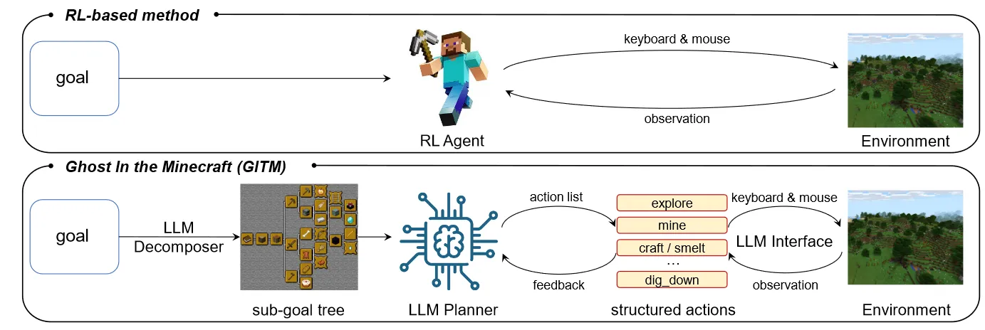
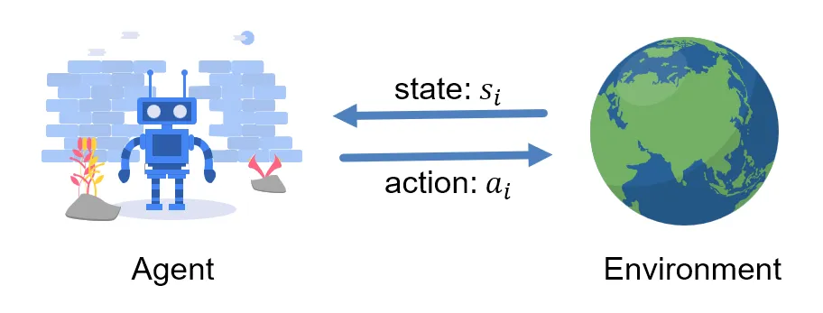
深度强化学习的流程可以抽象为以下步骤的重复：

1. 智能体与环境交互产生并存储经验
2. 智能体从经验中进行学习

本文主要探讨在收集经验过程中，环境自然结束（Terminated，包括目标成功，失败等）和人为截断（Truncated，主要为达到一定步数结束）对经验收集和训练产生的影响，以及如何对其进行处理。并对其进行了部分实验来比较性能。

The process of deep reinforcement learning can be abstracted into the following steps:

1. The agent interacts with the environment and generates and stores experiences.
2. The agent learns from the experiences.

This article mainly discusses the impact of natural termination (Terminated), including successful or failed goals, and artificial truncation (Truncated), mainly ending after a certain number of steps, on experience collection and training. It also conducts some experiments to compare performance.

现在是2023年5月17日凌晨00时57分，不知道是下午喝了那杯拿铁的缘故，还是因为这两天发生的事情，到现在依旧没有困意。此外，脑中也有很多想法在不断涌现和争辩。思来想去，与其在床上胡思乱想，亦或是借酒助眠，不如来工位写一篇文章，梳理一下脑中所想，将不断涌现的混乱的想法整理为有条理与逻辑的文本内容。

红豆生南国，春来发几枝？

愿君多采撷，此物最相思。

Now it is 00:57 on May 17, 2023. I still can't fall asleep, maybe because of the latte I had in the afternoon or because of what has happened in the past few days. My mind is filled with thoughts and debates. Instead of lying in bed and overthinking or relying on alcohol to fall asleep, I decided to write an article at my desk to organize my thoughts and turn the chaotic ideas into logical and organized text.

Red beans grow in the southern land, how many branches bloom in spring?

May you pick many, for this is the most lovesick thing.

强化学习在算法实现时需要非常注意细节，否则网络很难收敛或没有训练效果。本文主要记录我在实现各种强化学习算法时踩到的一些坑以及需要注意的细节，持续更新......

以及附上我自己实现的RL算法库：https://github.com/KezhiAdore/RL-Algorithm

Common

• Be cautious when implementing reinforcement learning algorithms, as attention to detail is crucial for convergence and training effectiveness. This article mainly documents some pitfalls encountered and details to be aware of while implementing various reinforcement learning algorithms, with continuous updates...

And here's my self-implemented RL algorithm library: https://github.com/KezhiAdore/RL-Algorithm

本文主要对于交叉熵的手动计算和PyTorch中的CrossEntropyLoss模块计算结果不一致的问题展开讨论，查阅了PyTorch的官方文档，最终发现是CrossEntropyLoss在计算交叉熵之前会对输入的概率分布进行一次SoftMax操作导致的。

This article mainly discusses the inconsistency between the manual calculation of cross-entropy and the results obtained by the CrossEntropyLoss module in PyTorch. After consulting the official documentation of PyTorch, it was found that the inconsistency was caused by the SoftMax operation performed by CrossEntropyLoss on the input probability distribution before calculating the cross-entropy.

In reinforcement learning, the loss function commonly used in policy learning is \(l=-\ln\pi_\theta(a|s)\cdot g\), where \(\pi_\theta\) is a probability distribution over actions given state \(s\), and \(a\) is the action selected in state \(s\). Therefore, we have:

\[ -\ln\pi_\theta(a|s) = -\sum_{a'\in A}p(a')\cdot \ln q(a') \]

\[ p(a') = \left\{ \begin{array}{lr} 1 &&& a'=a\\ 0 &&& otherwise \end{array} \right. \]

\[ q(a') = \pi_\theta(a'|s) \]

Thus, this loss function is transformed into the calculation of cross-entropy between two probability distributions. Therefore, we can use the built-in torch.nn.functional.cross_entropy function (referred to as the F.cross_entropy function below) in PyTorch to calculate the loss function. However, in practice, it was found that the results calculated using this function were inconsistent with the results calculated manually, which led to a series of investigations.

Firstly, we used Python to manually calculate the cross-entropy of two sets of data and the cross-entropy calculated using the F.cross_entropy function, as shown in the code below:

1
2
3
4
5
6
7
8
9
10
11
12
13

import torch
from torch.nn import functional as F

x = torch.FloatTensor([[0.4, 0.6],
                       [0.7, 0.3]])
y = torch.LongTensor([0, 1])

loss_1 = -torch.log(x.gather(1, y.view(-1,1)))
loss_2 = F.cross_entropy(x, y, reduction = "none")

print("Manually calculated cross-entropy:\n{}".format(loss_1.squeeze(1)))
print()
print("CrossEntropyLoss calculated cross-entropy:\n{}".format(loss_2))

The results of the above code are as follows:

1
2
3
4
5

Manually calculated cross-entropy:
tensor([0.9163, 1.2040])

CrossEntropyLoss calculated cross-entropy:
tensor([0.7981, 0.9130])

From the results, it can be seen that the two calculation results are not consistent. Therefore, we consulted the official documentation of PyTorch to understand the implementation of F.cross_entropy.

The description of the F.cross_entropy function in the documentation does not include the specific calculation process, only explaining the correspondence between the input data and the output result dimensions ¹. However, there is a sentence in the introduction of this function:

See CrossEntropyLoss for details.

So we turned to the documentation of CrossEntropyLoss ² and finally found the calculation process of cross-entropy in PyTorch:

It can be seen that the official documentation on the calculation of cross-entropy is very clear. In summary, the F.cross_entropy function requires at least two parameters, one is the predicted probability distribution, and the other is the index of the target true class. The important point is that the F.cross_entropy function does not require the input probability distribution to sum to 1 or each item to be greater than 0. This is because the function performs a SoftMax operation on the input probability distribution before calculating the cross-entropy.

Performing the SoftMax operation before calculating the cross-entropy improves the tolerance of the input, but if the SoftMax operation has been performed before the output is constructed in the neural network, it will cause the calculation of loss to be distorted, that is, the calculation results of the previous section are inconsistent.

According to the official documentation of PyTorch, if we add a SoftMax operation to the manual calculation of cross-entropy, we can get the same calculation result as the F.cross_entropy function. The following code is used to verify this:

1
2
3
4
5
6
7
8
9
10
11
12
13

import torch
from torch.nn import functional as F

x = torch.FloatTensor([[0.4, 0.6],
                       [0.7, 0.3]])
y = torch.LongTensor([0, 1])

loss_1 = -torch.log(F.softmax(x, dim=-1).gather(1, y.view(-1,1)))
loss_2 = F.cross_entropy(x, y, reduction = "none")

print("Manually calculated cross-entropy:\n{}".format(loss_1.squeeze(1)))
print()
print("CrossEntropyLoss calculated cross-entropy:\n{}".format(loss_2))

The output of the above code is as follows:

1
2
3
4
5

Manually calculated cross-entropy:
tensor([0.7981, 0.9130])

CrossEntropyLoss calculated cross-entropy:
tensor([0.7981, 0.9130])

Reference

最近在逐一复现RL算法过程中，策略梯度算法的收敛性一直有问题。经过一番探究和对比实验，学习了网上和书本上的很多实验代码之后，发现了代码实现中的一个小问题，即Policy Gradient在计算最终loss时求平均和求和对于网络训练的影响，本文将对此进行展开讨论。

先说结论：

在进行策略梯度下降优化策略时，可以对每个动作的loss逐一（for操作）进行反向传播后进行梯度下降，也可以对每个动作的loss求和（sum操作）之后进行反向传播后梯度下降，但尽量避免对所有动作的loss求平均（mean操作）之后进行反向传播后梯度下降，这会导致收敛速度较慢，甚至无法收敛。

具体的论证和实验过程见下文。