Digital Image Processing (Part 4) Spatial Domain Low-pass Filters.
This is an automatically translated post by LLM. The original post is in Chinese. If you find any translation errors, please leave a comment to help me improve the translation. Thanks!
Low-pass filters are very useful in our daily lives. Image blurring, image denoising, and image recognition all require the use of low-pass filters. Low-pass filtering means removing the high-frequency components (rapidly changing parts) from an image and leaving the low-frequency components (parts with less noticeable changes). There are two implementations of filters: spatial domain and frequency domain. Spatial domain filters operate directly on the spatial image, convolving the image matrix with the filter kernel to obtain the filtered output. Frequency domain filters transform the image to the frequency domain using the Fourier transform and then multiply it with the filter to obtain the output.
This article mainly introduces spatial domain low-pass filters and their implementations.
Commonly used spatial domain filters include average filtering, median filtering, and Gaussian filtering. Here, we mainly introduce median filtering and Gaussian filtering.
Median Filtering
As the name suggests, median filtering is a filter based on statistical methods. The specific implementation method is as follows: for an n*n median filter, the pixel value of the output image at (x, y) is equal to the median of all pixel values in the n*n image area centered at (x, y) in the input image.
The size of the filter can be selected according to different needs.
The effect of the median filter is as follows:
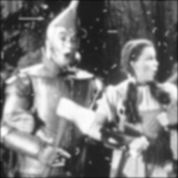
The original image, 3*3 median filter, 5*5 median filter, and 7*7 median filter, respectively.
 Original Image Original Image
|
 3*3
Median Filter 3*3
Median Filter
|
 5*5
Median Filter 5*5
Median Filter
|
 7*7
Median Filter 7*7
Median Filter
|
The original image contains a lot of irregularly distributed noise, some of which are salt noise, but most of them are sudden impulse noise. When using a 3*3 median filter, the salt noise has been removed well, but the impulse noise is still obvious. When using a 5*5 median filter, the situation of impulse noise has been greatly improved. The 7*7 filter almost completely removes the noise, but the image is also severely blurred.
Gaussian Filtering
Gaussian filtering is a commonly used blurring method in some image processing software. It is generated by the two-dimensional normal distribution function: \(p(x,y)=\frac1{2\pi\sigma^2}e^{-\frac{x^2+y^2}{2\sigma^2}}\). The specific steps are as follows:
- To generate an n*n Gaussian filter, set the center of the n-order simulation to (0,0) and generate the coordinates of other positions in the matrix.
- Substitute the coordinates of each position in the n*n matrix into the two-dimensional normal distribution function to obtain the value of each position.
- Scale the values in the matrix based on the value of 1 in the upper left corner of the matrix.
- Round the matrix to obtain the n*n Gaussian filter.
The function for generating a Gaussian filter is as follows:
2
3
4
5
6
7
8
9
10
11
12
sigma=1.5 # Parameter of the Gaussian filter
def f(x,y): # Define the two-dimensional normal distribution function
return 1/(math.pi*sigma**2)*math.exp(-(x**2+y**2)/(2*sigma**2))
def gauss(n): # Generate an n*n Gaussian filter
mid=n//2
filt=np.zeros((n,n))
for i in range(n):
for j in range(n):
filt[i][j]=f(i-mid,j-mid)/f(-mid,-mid)
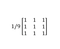
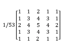
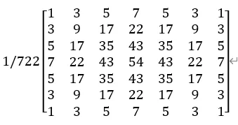
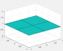
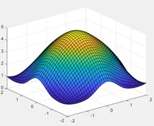
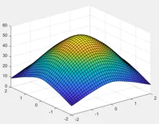
return filt.astype(np.uint8)The Gaussian filters of size 3*3, 5*5, and 7*7 are as follows:
Their images in the two-dimensional coordinate system are as follows:
After obtaining the operator of the Gaussian filter, convolve it with the input image to obtain the result of the Gaussian filter.
The effect is as follows:
The original image, 3*3, 5*5, and 7*7 Gaussian filtering results:
|
Original Image
|
 3*3
Gaussian 3*3
Gaussian
|
 5*5
Gaussian 5*5
Gaussian
|
 7*7
Gaussian 7*7
Gaussian
|
Gaussian blur is more effective in removing salt noise in the image, but it is more difficult to remove impulse noise. The 7*7 Gaussian filter still cannot remove the impulse noise in the image. On the other hand, compared with Gaussian blur, Gaussian blur retains more information of the image and preserves more details.
Appendix
References
[1] Digital Image Processing, Third Edition / (Rafael C. Gonzalez), translated by Ruan Qiuqi, et al. - Beijing: Electronic Industry Press, 2017.5
[2] Brook_icv. Basic Image Processing (4): Detailed Explanation of Gaussian Filters [G/OL]. Blog Garden: 2017-02-16 [2020-03-23]. https://www.cnblogs.com/wangguchangqing/p/6407717.html#autoid-4-1-0
[3] Yu Ni Xin An. Methods for Calculating Mean, Median, and Mode in Numpy [G/OL]. Blog Garden: 2018-11-04 [2020-03-23]. https://www.cnblogs.com/lijinze-tsinghua/p/9905882.html
Source Code
1 | import cv2 as cv |


.jpg?x-oss-process=style/webp)