Crawling all anime data from Bilibili and conducting data analysis.

This is an automatically translated post by LLM. The original post is in Chinese. If you find any translation errors, please leave a comment to help me improve the translation. Thanks!

Introduction

Bilibili (referred to as B station) has a large number of anime copyrights, with a total of 3161 as of now. Each anime can be found with its play count, follow count, barrage count, and other playback data. In addition, each anime has its corresponding tags (such as "comic adaptation", "hot-blooded", "comedy"). This project aims to analyze the relationship between anime playback data and anime tags, and it is also a data analysis project that uses APriori frequent itemset mining for analysis.

GitHub address: https://github.com/KezhiAdore/BilibiliAnimeData_Analysis

Gitee address: https://gitee.com/KezhiAdore/BilibiliAnimeData_Analysis

Data Collection

First, we need to obtain all the data we need, which are all the anime playback information and tag information on B station. We use web crawlers to crawl the data, and here we use scrapy in Python to write the crawler to crawl the data.

Page Analysis

First, go to the anime index page on B station

Click on a certain anime on this page to enter its details page

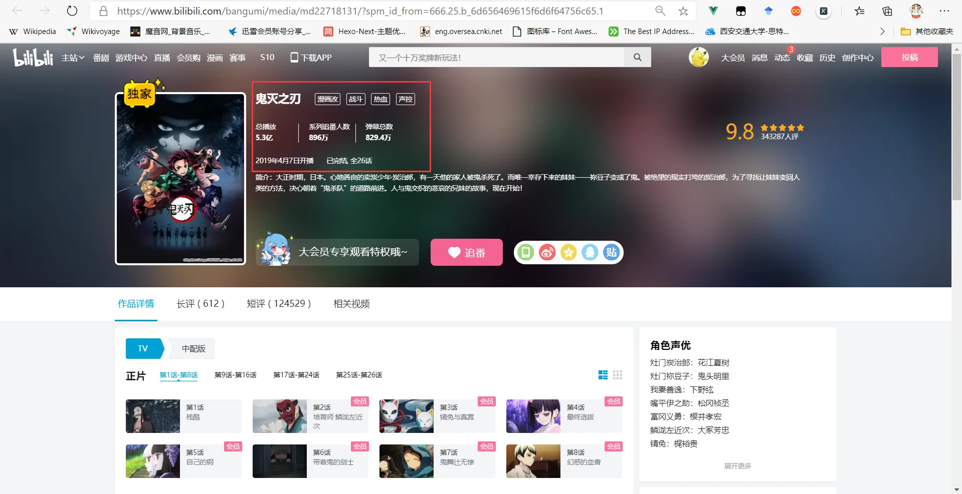
You can see that the required anime playback data and anime tags are available on this page.

Analyze the HTML of this page to find the xpath path where the data is located, taking tags as an example:

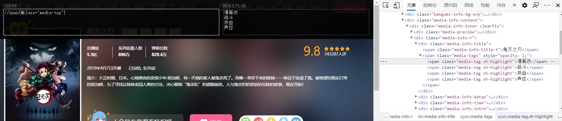
The xpath paths corresponding to all the data are:

Tags: //span[@class="media-tag"]
Total Plays: //span[@class="media-info-count-item media-info-count-item-play"]/em
Follow Count: //span[@class="media-info-count-item media-info-count-item-fans"]/em
Barrage Count: //span[@class="media-info-count-item media-info-count-item-review"]/em

So far, we can loop through all the anime list pages, enter the details page from this page, and parse each anime details page to save the data. However, there is a problem at this point. After crawling the anime list page, the corresponding place in the web page data is:

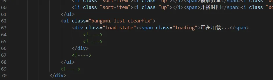
Directly accessing this page cannot obtain detailed anime list information. Therefore, we need to analyze the files received by the page and find the anime list information obtained by this page.

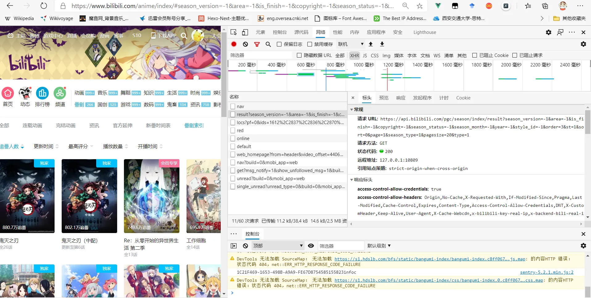
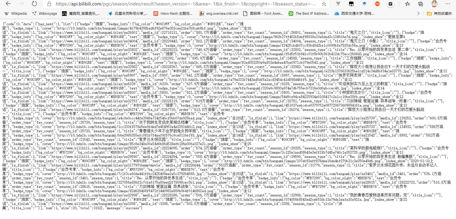
Accessing this URL will get the following information:

Analyzing this API URL, it can be found that the page=1 controls the page number information, and by changing this information, different anime list pages can be accessed.

https://api.bilibili.com/pgc/season/index/result?season_version=-1&area=-1&is_finish=-1&copyright=-1&season_status=-1&season_month=-1&year=-1&style_id=-1&order=3&st=1&sort=0&page=1&season_type=1&pagesize=20&type=1

The information obtained from this page is a JSON file, and the information format is as follows:

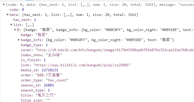
By comparing with the URL of the anime details page https://www.bilibili.com/bangumi/media/md22718131, it can be found that the media_id data in the JSON file is the identifier of each anime details page. Therefore, the logic of crawling information is basically established.

1. Access the initial API page (page=1), parse its content, and get the media_id of all anime on this page.
2. Use media_id to construct the link to access the anime details page, crawl this page for parsing, and get the data of an anime.
3. Access the next API page and repeat the above steps.

Spider Construction

First, initialize the spider

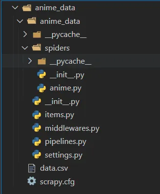
scrapy startproject anime_data
scrapy genspider anime ""

The file tree is as follows

Open items.py and create the data object that needs to be saved

import scrapy

class AnimeDataItem(scrapy.Item):
    # define the fields for your item here like:
    name = scrapy.Field()   # Anime name
    play=scrapy.Field()     # Total play count
    fllow=scrapy.Field()    # Follow count
    barrage=scrapy.Field()  # Barrage count
    tags=scrapy.Field()     # Anime tags, in list format
    pass

Then open the newly created anime.py, access the page, parse it, and save the data as follows

import scrapy
import json
from anime_data.items import AnimeDataItem

class AnimeSpider(scrapy.Spider):
    name = 'anime'
    #allowed_domains = ['https://www.bilibili.com']
    # Anime information table API
    url_head="https://api.bilibili.com/pgc/season/index/result?season_version=-1&area=-1&is_finish=-1&copyright=-1&season_status=-1&season_month=-1&year=-1&style_id=-1&order=3&st=1&sort=0&season_type=1&pagesize=20&type=1"
    start_urls = [url_head+"&page=1"]

## Recursive parsing of anime information table
    def parse(self, response):
        data=json.loads(response.text)
        next_index=int(response.url[response.url.rfind("=")+1:])+1
        if data['data']['size']==20:
            next_url=self.url_head+"&page="+str(next_index)
            yield scrapy.Request(next_url,callback=self.parse)
        for i in data['data']['list']:
            media_id=i['media_id']
            detail_url=("https://www.bilibili.com/bangumi/media/md"+str(media_id))
            yield scrapy.Request(detail_url,callback=self.parse_detail)
        pass

## Parse anime details page
    def parse_detail(self,response):
        item=AnimeDataItem()
        # Anime name
        item['name']=response.xpath('//span[@class="media-info-title-t"]/text()').extract()[0]
        # Play count
        item['play']=response.xpath('//span[@class="media-info-count-item media-info-count-item-play"]/em/text()').extract()[0]
        # Follow count
        item['fllow']=response.xpath('//span[@class="media-info-count-item media-info-count-item-fans"]/em/text()').extract()[0]
        # Barrage count
        item['barrage']=response.xpath('//span[@class="media-info-count-item media-info-count-item-review"]/em/text()').extract()[0]
        # Anime tags
        item['tags']=response.xpath('//span[@class="media-tag"]/text()').extract()
        return item

Data Analysis

Data Cleaning and Filtering

The collected data cannot be used directly and needs to be cleaned and filtered, which can be divided into two steps:

1. Remove data without tag information
2. Convert quantity information in the data to numbers (e.g., convert "10,000" to "10000")

For the first step, since the data volume is small, you can quickly complete it using the filtering function in Excel.

For the second step, write the following function to convert the data:

# Convert text data to numbers
def trans(string):
    if string[-1]=='万':
        return int(float(string[0:-1])*1e4)
    elif string[-1]=='亿':
        return int(float(string[0:-1])*1e8)
    else:
        return int(string)

Frequent Itemset Mining using Apriori Algorithm

1. Itemsets and Datasets

Let the set of all items appearing in the data be \(U=\left\{I_1,I_2,...,I_n\right\}\), and let the data to be mined for frequent itemsets be the set of transactions in the database \(D\). The data in \(D\) are itemsets, and each itemset \(T\subseteq U\).

2. Association Rules (Support and Confidence)

Let \(A\) and \(B\) be two itemsets, \(A\subset U,B\subset U, A\neq \emptyset，B\neq \emptyset，A\cap B=\emptyset\).

An association rule is in the form of \(A\Rightarrow B\), and its support in the transaction set \(D\) is denoted as \(s\), where \(s\) is the percentage of transactions in the transaction set \(D\) that contain \(A\cup B\).

Its confidence in the transaction set \(D\) is denoted as \(c\), which is the percentage of transactions in the transaction set \(D\) that contain \(B\) among the transactions that contain \(A\), i.e., \(P(A|B)\). \[ c=P(B|A)=\frac{P(A\cup B)}{P(A)}=\frac{support(A\cup B)}{support(A)}=\frac{support\text{_}count(A\cup B)}{support\text{_}count(A)} \]

3. Frequent Itemsets

When mining frequent itemsets, set the minimum confidence and minimum support, and rules that satisfy both the minimum support and minimum confidence are called strong rules, and itemsets that satisfy such strong rules are called frequent itemsets.

Association Rules

Each anime has a certain number of tags to roughly describe its content. The tags used to describe the same anime are usually descriptions in different dimensions. Taking "Miss Kobayashi's Dragon Maid" as an example, its tags are [moe, comedy, daily life, comic adaptation], and the four tags describe four different characteristics of this anime. By analyzing the anime tag data on B station, find the combinations of tags with the highest relevance.

Algorithm Flow

Data set: The tag data set of all anime, each data is the tag of an anime

The flow of the Apriori algorithm is as follows:

1. Construct 1-itemsets -> Count the frequency of 1-itemsets -> Calculate support and confidence -> Pruning -> Frequent 1-itemsets

2. Construct k-itemsets using k-1-itemsets -> Count the frequency of k-itemsets -> Calculate support and confidence -> Pruning -> Frequent k-itemsets

3. Repeat step 2 until there are no itemsets that meet the strong rules

Programming Implementation

First, read the processed data and convert the tag data, which is originally a string, into a list:

filepath='data_processed.csv'
df=pd.read_csv(filepath)
tags=df['tags'].to_list()

The data in tags is a string rather than a list, such as: "恋爱,推理,校园,日常", which needs to be converted into a list. The implementation is as follows:

# Convert comma-separated strings to lists using commas as separators
def str_to_list(str_data):
    for index,data in enumerate(str_data):
        tmp,start,end=[],0,0
        while end!=len(data):
            if data[start:].find(',')==-1:
                end=len(data)
                tmp.append(data[start:end])
                break
            end=start+data[start:].find(',')
            tmp.append(data[start:end])
            start=end+1
        str_data[index]=tmp

Construct k-itemsets using k-1-itemsets:

# Apriori algorithm connection step, implemented step by step
def merge_list(l1,l2):
    length=len(l1)
    for i in range(length-1):
        if l1[i]!=l2[i]:
            return 'nope'
    if l1[-1]<l2[-1]:
        l=l1.copy()
        l.append(l2[-1])
        return l
    else:
        return 'nope'

Determine the inclusion relationship between lists:

# Determine if l2 is included in l1
def is_exist(l1,l2):
    for i in l2:
        if i not in l1:
            return False
    return True

Pruning operation:

# Prune using min_sup and min_conf, that is, minimum support and minimum confidence, L_last is the frequent k-1-itemset
def prune(L=[],L_last=0,min_sup=0,min_conf=0):
    tmp_L=[]
    if L_last==0 or min_conf==0:
        for index,l in enumerate(L):
            if l[1]<min_sup:
                continue
            tmp_L.append(l)
    else:
        for index,l in enumerate(L):
            if l[1]<min_sup:
                continue
            for ll in L_last:
                if l[0][:-1]==ll[0]:
                    if l[1]/ll[1]>=min_conf:
                        tmp_L.append(l)
    return tmp_L

Apriori algorithm main body:

def Apriori(data,min_sup,min_conf):
    # C: Temporary storage for k-itemsets  L: Temporary storage for frequent k-itemsets  L_save: Save frequent 1-k-itemsets
    C,L,L_save=[],[],[]
    # Use support count instead of support for calculation
    min_sup_count=min_sup*len(data)
    # Initialize 1-itemsets
    for tags in data:
        for tag in tags:
            if C==[] or [tag] not in[x[0] for x in C]:
                C.append([[tag],0])
    # Filter out frequent 1-itemsets
    L=C.copy()
    for index,l in enumerate(L):
        for tags in data:
            if is_exist(tags,l[0]):
                L[index][1]+=1
    L=prune(L,min_sup=min_sup)
    L_save.append(L)
    while True:
        # Construct k-itemsets using k-1-itemsets
        C=[]
        for l1 in L:
            for l2 in L:
                list_merge=merge_list(l1[0],l2[0])
                if list_merge!='nope':
                    C.append([list_merge,0])
        # Count frequency and prune
        L=C.copy()
        for index,l in enumerate(L):
            for tags in data:
                if is_exist(tags,l[0]):
                    L[index][1]+=1
        L=prune(L,L_save[-1],min_sup,min_conf)
        # End the loop when L is an empty set
        if L==[]:
            return L_save
        L_save.append(L)

K-means Clustering Algorithm

Algorithm Introduction

K-means is an unsupervised clustering algorithm. The algorithm is simple and easy to implement, but it may produce empty clusters or converge to local optima.

The algorithm flow is as follows:

1. Randomly select k points from the samples as initial centroids.
2. Calculate the distance from each sample to these k centroids and assign the sample to the cluster whose centroid is closest to it.
3. Recalculate the centroids of each cluster.
4. Repeat steps 2 and 3 until the centroids do not change.

Data Mapping

Use K-means to cluster the anime based on the three-dimensional coordinates formed by the three types of data [play count, follow count, barrage count]. However, the values of these three data range from thousands to billions, so they cannot be used directly. Apply a logarithmic function to compress the data: \[ [x,y,z]=[ln\ x,ln\ y,ln\ z] \] After the logarithmic transformation, in order to ensure that each type of data has the same range to ensure that they have the same weight, normalize the data: \[ x=\frac{x-min}{max-min} \] The implementation code is as follows:

def trans_data(data):
    for index,item in enumerate(data):
        data[index]=math.log(item)
    Max=max(data)
    Min=min(data)
    for index,item in enumerate(data):
        data[index]=(item-Min)/(Max-Min)

K-means Programming Implementation

In clustering, the distance measure used is the Euclidean distance, which is: \[ distance=\sqrt{(x_{1}-y_{1})^2+...+(x_{i}-y_{i})^2+...+(x_{n}-y_{n})^2} \] The implementation code is as follows:

def distance(point1,point2):
    dim=len(point1)
    if dim != len(point2):
        print('error! dim of point1 and point2 is not same')
    dist=0
    for i in range(dim):
        dist+=(point1[i]-point2[i])*(point1[i]-point2[i])
    return math.sqrt(dist)

1. Randomly select k points as centroids

shape=np.array(dire).shape
    k_center_index=[]
    k_center=[]
    temp_k=k
    while(temp_k):
        temp=random.randrange(0,shape[0])
        if temp not in k_center_index:
            k_center_index.append(temp)
            k_center.append(list(dire[temp]))
            temp_k-=1

2. Cluster all the data

def get_category(dire,k,k_center):
    shape=np.array(dire).shape
    k_categories=[[] for col in range(k)]
    for i in range(shape[0]):
        Min=1
        for j in range(k):
            dist=distance(dire[i],k_center[j])
            if dist<Min:
                Min=dist
                MinNum=j
        k_categories[MinNum].append(i)
    return k_categories

3. Calculate new centroids and repeat

# Maximum number of iterations
    Maxloop=500
    k_center_new=k_center
    k_center=[]
    count=0
    while(k_center!=k_center_new and count<Maxloop):
        count+=1
        k_center=copy.deepcopy(k_center_new)
        k_categories=get_category(dire,k,k_center_new)
        for i in range(shape[1]):
            for j in range(k):
                temp=0
                for w in k_categories[j]:
                    temp+=dire[w][i]
                k_center_new[j][i]=temp/len(k_categories[j])

The complete K-means algorithm main body is as follows:

def k_means(dire,k):
    # Randomly select k points as centroids
    shape=np.array(dire).shape
    k_center_index=[]
    k_center=[]
    temp_k=k
    while(temp_k):
        temp=random.randrange(0,shape[0])
        if temp not in k_center_index:
            k_center_index.append(temp)
            k_center.append(list(dire[temp]))
            temp_k-=1

    # Maximum number of iterations
    Maxloop=500
    k_center_new=k_center
    k_center=[]
    count=0
    while(k_center!=k_center_new and count<Maxloop):
        count+=1
        k_center=copy.deepcopy(k_center_new)
        k_categories=get_category(dire,k,k_center_new)
        for i in range(shape[1]):
            for j in range(k):
                temp=0
                for w in k_categories[j]:
                    temp+=dire[w][i]
                k_center_new[j][i]=temp/len(k_categories[j])
    return {'k_center':k_center,'k_categories':k_categories,'dire':dire,'k':k}

Algorithm Results and Evaluation

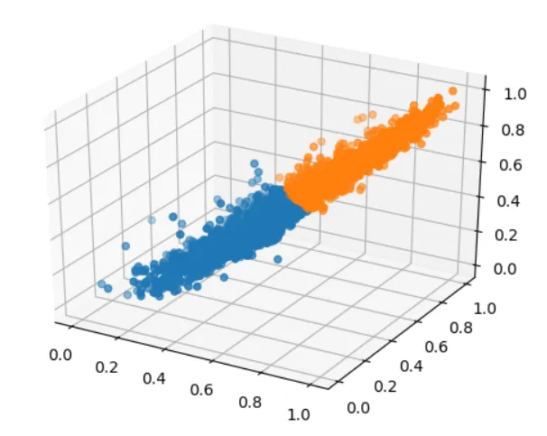
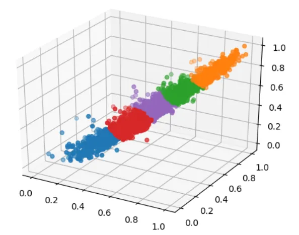
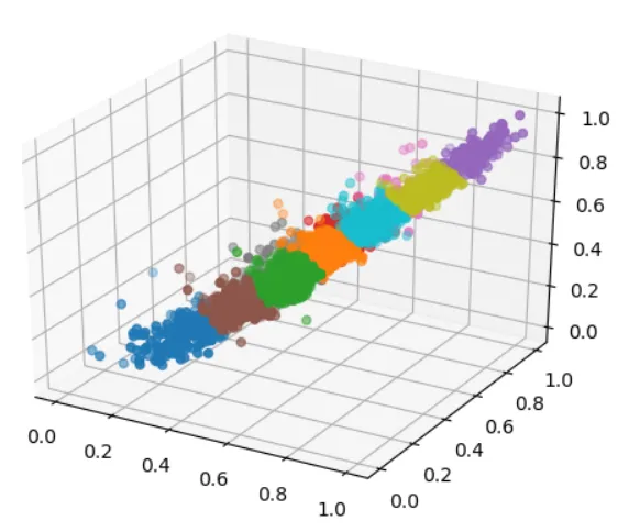
To visually see the clustering results, plot the clustered points in three-dimensional space, using different colors to represent different categories.

The plotting function is as follows:

def show_k_means(k_result):
    k,k_categories,dire=k_result['k'],k_result['k_categories'],k_result['dire']
    for i in range(k):
        x,y,z=[],[],[]
        for index in k_categories[i]:
            x.append(dire[index][0])
            y.append(dire[index][1])
            z.append(dire[index][2])
        fig = plt.gcf()
        ax = fig.gca(projection='3d')
        ax.scatter(x,y,z)
    plt.show()

The clustering results are as follows:

k=2	k=5	k=10

To evaluate the clustering effect, select the Davies-Bouldin Index (DBI) to evaluate the clustering effect. The algorithm and method of DBI are as follows:

• Suppose there are k clusters, and the center point of each cluster is \(u_i\), and the points in the cluster are represented by \(x_{ij}\)
• Calculate the average distance within each cluster \(\mu_i\), which is the average distance from all points in the cluster to the cluster center
• Calculate the distance between centroids \(d(u_i,u_j)\)
• Calculate DBI:

\[ DB=\frac1k\sum_{i=1}^k\mathop{max}\limits_{i\neq j}(\frac{\mu_i+\mu_j}{d(u_i,u_j)}) \]

The implementation code is as follows:

def dbi(k_result):
    k_center,k_categories,dire,k=k_result['k_center'],k_result['k_categories'],k_result['dire'],k_result['k']
    # Average distance within clusters
    k_ave_dist=[0 for index in range(k)]
    for i in range(k):
        temp=0
        for item in k_categories[i]:
            temp+=distance(k_center[i],dire[item])
        k_ave_dist[i]=temp/len(k_categories[i])
    # Distance between cluster centers
    k_center_dist=[[0 for row in range(k)] for col in range(k)]
    for i in range(k):
        for j in range(k):
            k_center_dist[i][j]=distance(k_center[i],k_center[j])
    # Calculate DBI
    DB=0
    for i in range(k):
        Max=0
        for j in range(k):
            if i !=j:
                temp=(k_ave_dist[i]+k_ave_dist[j])/k_center_dist[i][j]
                if temp>Max:
                    Max=temp
        DB+=Max
    return DB/k

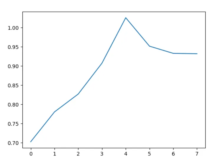
The evaluation results of clustering when k=2-10 are as follows:

k	2	3	4	5	6	7	8	9	10
DBI	0.7028	0.7851	0.8324	0.9075	0.9267	0.9927	0.9242	0.9123	0.8849

The evaluation results of k=2-50 are as follows:

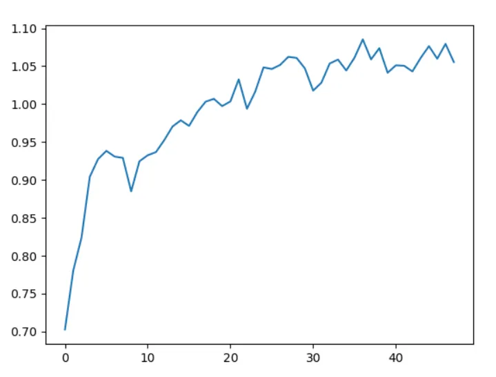
From the above results, it can be seen that the clustering effect is best when k=2 or 3. Analyzing from the data used and the characteristics of the k-means algorithm, the k-means algorithm uses Euclidean distance for clustering, and the regions divided are spherical. From the three-dimensional image, the data used does not have a clear boundary to separate the data. When k=2 or 3, each cluster is concentrated in a sphere, showing better clustering results. As k continues to increase, the clustering effect gradually deteriorates due to the influence of isolated points around the data.