Linear filtering and nonlinear filtering experiments.
This is an automatically translated post by LLM. The original post is in Chinese. If you find any translation errors, please leave a comment to help me improve the translation. Thanks!
This article presents experiments on linear filtering and nonlinear filtering for estimating the free fall motion. The following figure is from Professor Cai Yuanli's course "Random Filtering and Control" at Xi'an Jiaotong University. The course mainly discusses various filtering methods related to estimation, smoothing, and prediction.

Problem Description
A object is in free fall motion, and its height has been measured 20 times. The measurement values are shown in the following table:
Consider the same object in free fall motion, and use a radar (in the same horizontal plane as the object) for measurement. The measurement noise of radar range and angle is a Gaussian white noise sequence with a mean of 0 and a variance matrix \(R=\begin{bmatrix}0.04 &0\\0&0.01\end{bmatrix}\). Based on the following measurement data, determine the estimated values of the object's height and downward velocity over time:
The descent motion and radar detection information are shown in the following figure:
Model Introduction
1. Linear Estimation Problem
Assume that during free fall motion, the object's height is \(h\) and velocity is \(v\) (downward is positive). Let \(x_1=h\) and \(x_2=v\), then the system's state equation is:
\[ \begin{bmatrix} \dot x_1\\\dot x_2 \end{bmatrix}= \begin{bmatrix} 0&-1\\ 0&0\\ \end{bmatrix} \begin{bmatrix} x_1\\x_2 \end{bmatrix}+ \begin{bmatrix} 0\\1 \end{bmatrix}g\ \ (g=9.80m/s^2) \]
The state transfer function of the system can be solved from the above state equation:
\[ x(t)=\begin{bmatrix} 1&-t\\ 0&1 \end{bmatrix}x(0) +\begin{bmatrix} -t\\1 \end{bmatrix}u(t) \]
When the time step is 1s, the state transfer function of the system is:
\[ \Phi_{k+1,k}=\begin{bmatrix} 1&-1\\ 0&1 \end{bmatrix} \ \Psi_{k+1,k}=\begin{bmatrix} -1\\ 1 \end{bmatrix} \]
Therefore, the one-step prediction of the system is:
\[ x_{k+1,k}=\Phi_{k+1,k}x_{k|k}+\Psi_{k+1,k}u_k \]
Since the observation is a direct measurement of the object's height, and assuming the measurement error is a white noise with a mean of 0 and a variance of 1, the measurement equation is:
\[ y_k=H_kx_k+v_k \]
where:
\[ H_k\equiv \begin{bmatrix} 1\\0 \end{bmatrix}, \ v_k \sim N(0,1), \ R=1 \]
In this problem, the measurement height unit is \(km\), and the acceleration is \(9.8m/s^2\). For ease of calculation, the distance unit is unified to \(km\), and the time unit is unified to \(s\), so the gravity acceleration \(g=0.0098km/s\). Since the initial value of the filter is not given, the initial height is estimated as \(2km\) based on the measurement data, and the initial velocity is 0, i.e., \(x_{0|0}=\begin{bmatrix}2&0\end{bmatrix}\). Since the initial estimate value determined in this way is relatively rough, the variance is large. Therefore, the initial variance matrix of the system is set to \(P_{0|0}=\begin{bmatrix}10&0\\0&10\end{bmatrix}\).
Establish the Kalman filter equations: \[ x_{k+1,k}=\Phi_{k+1,k}x_{k|k}+\Psi_{k+1,k}u_k\\ P_{k+1|k}=\Phi_{k+1,k}P_{k|k}\Phi^\top_{k+1,k}\\ P_{k+1|k+1}=[P_{k+1|k}^{-1}+H_{k+1}^{\top} R_{k+1}^{-1}H_{k+1}]^{-1}\\ K_{k+1}=P_{k+1|k+1}H_{k+1}^\top R_{k+1}^{-1}\\ \hat x_{k+1|k+1}=\hat x_{k+1|k}+K_{k+1}(y_{k+1}-H_{k+1}\hat x_{k+1|k}) \] Calculate the descent height and velocity of the object, and the calculation results are shown in the experimental results section below.
2. Nonlinear Estimation Problem
In the second problem, the measurement and estimation values are nonlinearly related. Consider using the Extended Kalman Filter (EKF) algorithm to estimate it. In this report, the Extended Kalman Filter algorithm is used.
Let the measured slant range be \(l(km)\), the elevation angle be \(\theta(rad)\), the height of the object be \(h(km)\), and the downward velocity be \(v(km/s)\) (downward is positive). The vertical projection of the object on the ground to the radar is \(d_0\).
For ease of subsequent linearization calculations, the system state variables are selected as: \[ x_1=h,\ x_2=v,\ x_3=d_0 \] Then the system's state equation is: \[ \dot x= \begin{bmatrix} 0&-1&0\\ 0&0&0\\ 0&0&0 \end{bmatrix}x+ \begin{bmatrix} 0\\ 1\\ 0 \end{bmatrix}g,\ where\ g=0.0098\ km/s \] Solving the equation, when the time interval is \(0.5s\), the discrete state transfer function of the system is: \[ \Phi_{k+1,k}=\begin{bmatrix} 1&-0.5&0\\ 0&1&0\\ 0&0&1 \end{bmatrix},\ \Psi_{k+1,k}=\begin{bmatrix} -0.125\\ 0.5\\ 0 \end{bmatrix} \] The observation of the system is the slant range and elevation angle measured by the radar, then: \[ y_1=l=\sqrt{h^2+d_0^2}=\sqrt{x_1^2+x_3^2}\\ y_2=\theta=\arctan(\frac{h}{d_0})=\arctan(\frac{x_1}{x_3}) \] Taking the derivative of the observation with respect to the state variables, we have: \[ \frac{\partial y_1}{\partial x_1}=\frac{x_1}{\sqrt{x_1^2+x_3^2}}\\ \frac{\partial y_1}{\partial x_2}=0\\ \frac{\partial y_1}{\partial x_3}=\frac{x_3}{\sqrt{x_1^2+x_3^2}}\\ \frac{\partial y_2}{\partial x_1}=\frac{x_3}{x_1^2+x_3^2}\\ \frac{\partial y_2}{\partial x_2}=0\\ \frac{\partial y_2}{\partial x_3}=-\frac{x_1}{x_1^2+x_3^2}\\ \] Therefore, the local linearization coefficients of the system are: \[ H=\begin{bmatrix} \frac{x_1}{\sqrt{x_1^2+x_3^2}}&0&\frac{x_3}{\sqrt{x_1^2+x_3^2}}\\ \frac{x_3}{x_1^2+x_3^2}&0&-\frac{x_1}{x_1^2+x_3^2} \end{bmatrix} \] The calculation process of the Extended Kalman Filter (EKF) is as follows: \[ x_{k+1,k}=\Phi_{k+1,k}x_{k|k}+\Psi_{k+1,k}u_k\\ P_{k+1|k}=\Phi_{k+1,k}P_{k|k}\Phi^\top_{k+1,k}\\ P_{k+1|k+1}=[P_{k+1|k}^{-1}+H_{k+1}^{\top} R_{k+1}^{-1}H_{k+1}]^{-1}\\ K_{k+1}=P_{k+1|k+1}H_{k+1}^\top R_{k+1}^{-1}\\ \hat x_{k+1|k+1}=\hat x_{k+1|k}+K_{k+1}(y_{k+1}-H_{k+1}\hat x_{k+1|k}) \] The difference between the Extended Kalman Filter and the Kalman Filter is that the coefficient matrix \(H\) is obtained by local linearization at the observation point. With the above steps, the nonlinear observation can be filtered and estimated.
Experimental Results
1. Linear Filtering Problem
Based on the given height observation data, linear Kalman filtering is performed, and the calculated results are as follows:
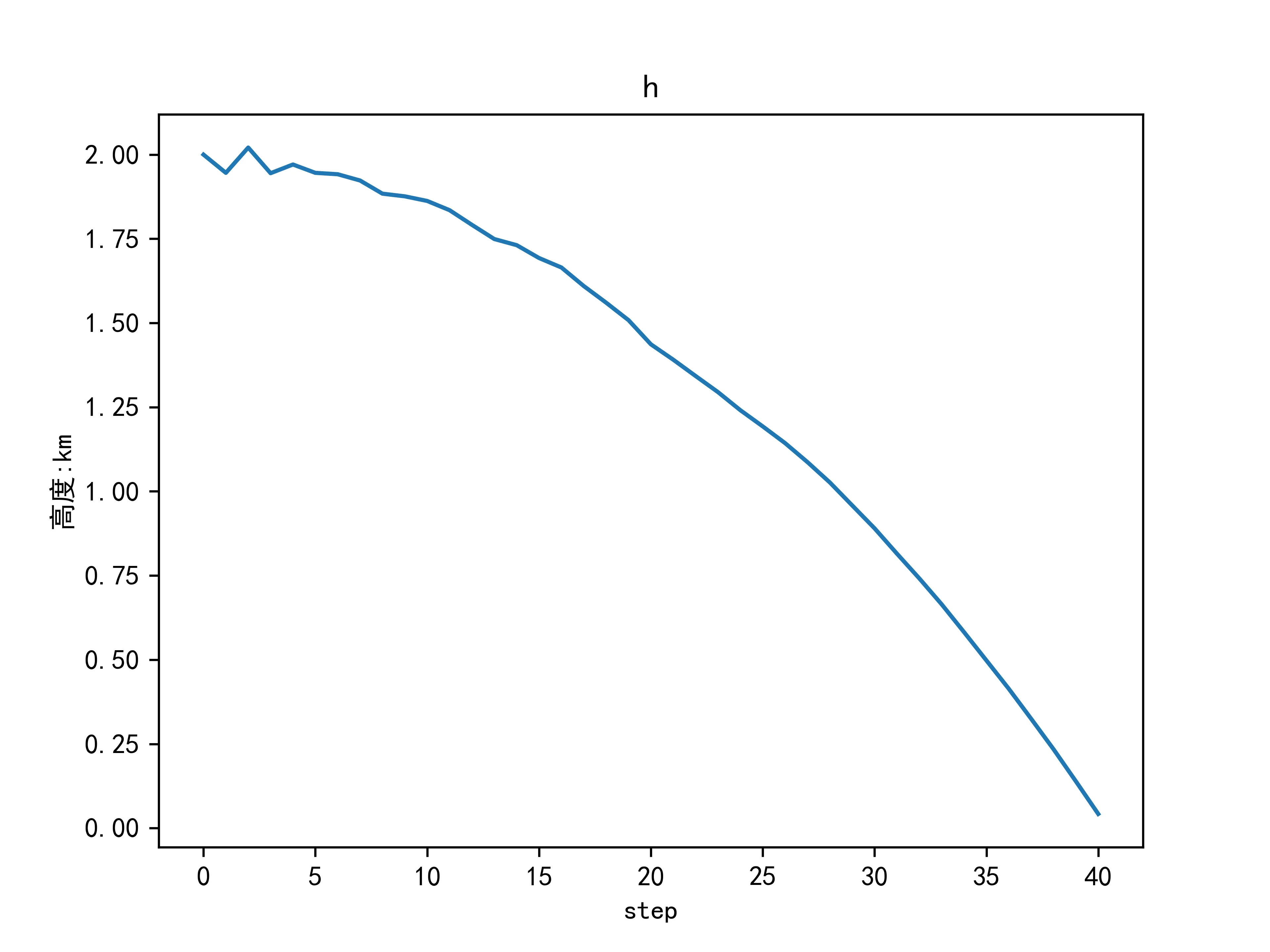
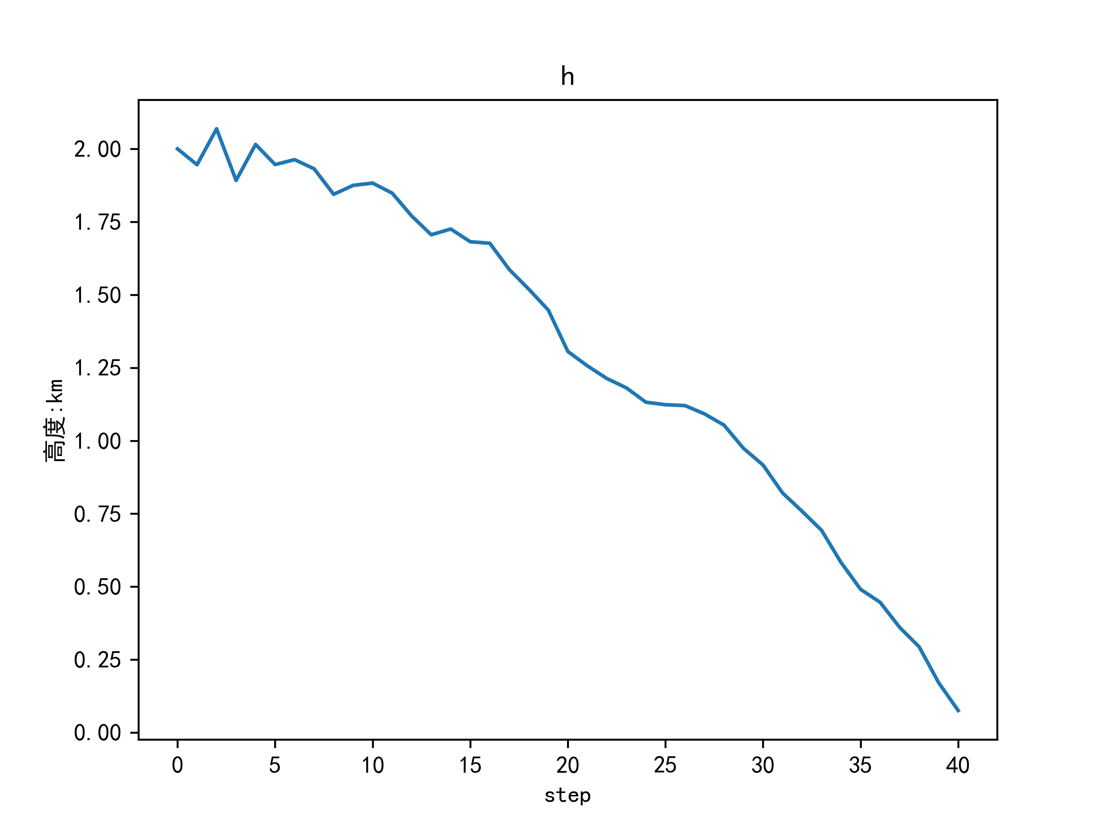
The estimated height data is:
| Time | 1 | 2 | 3 | 4 | 5 | 6 | 7 |
|---|---|---|---|---|---|---|---|
| Height | 1.9943 | 1.9791 | 1.9550 | 1.9211 | 1.8774 | 1.8244 | 1.7605 |
| Time | 8 | 9 | 10 | 11 | 12 | 13 | 14 |
|---|---|---|---|---|---|---|---|
| Height | 1.6870 | 1.6038 | 1.5103 | 1.4075 | 1.2947 | 1.1723 | 1.0400 |
| Time | 15 | 16 | 17 | 18 | 19 | 20 | |
|---|---|---|---|---|---|---|---|
| Height | 0.8980 | 0.7460 | 0.5845 | 0.4129 | 0.2317 | 0.0405 |
The height change graph is shown below:

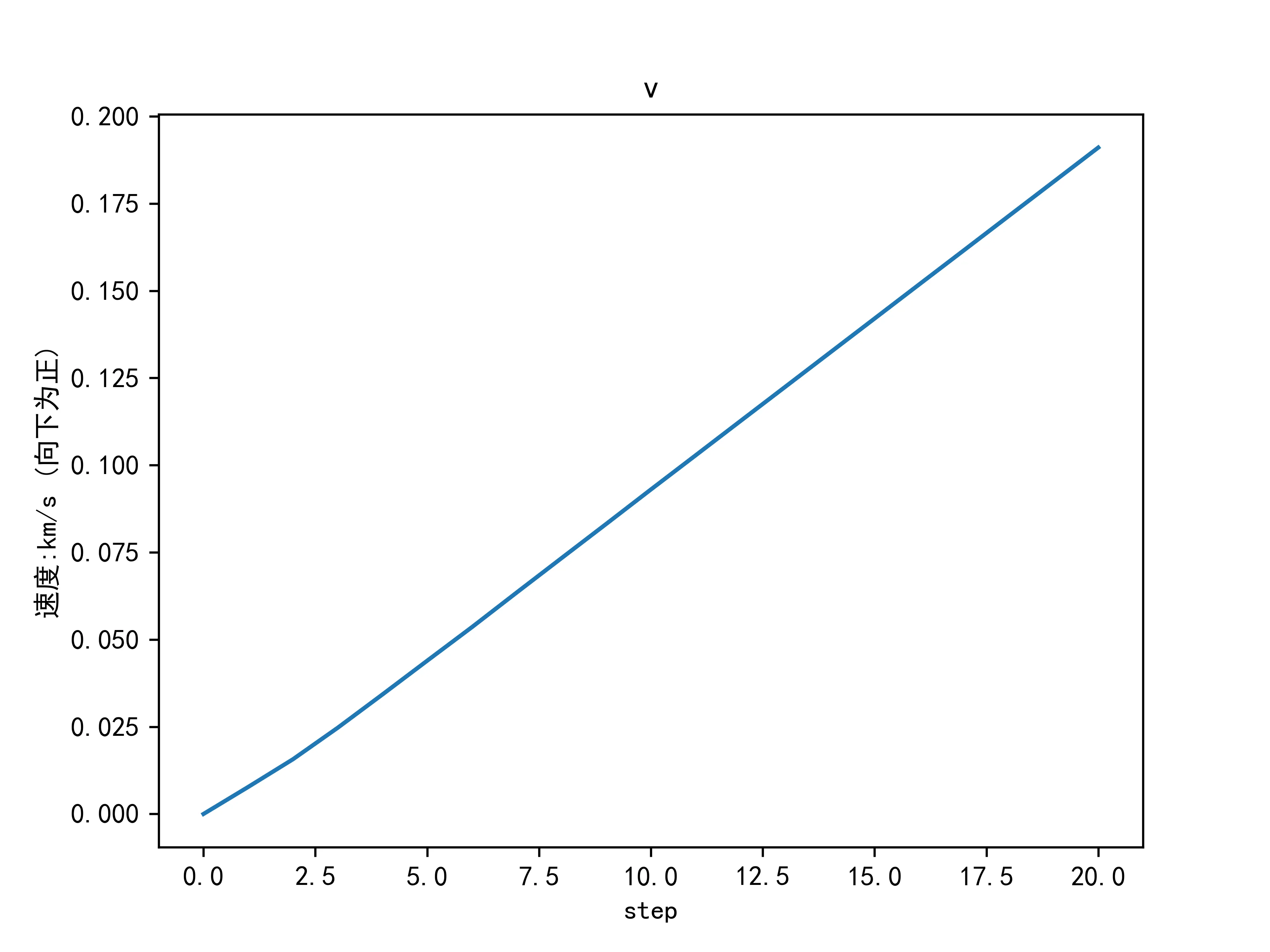
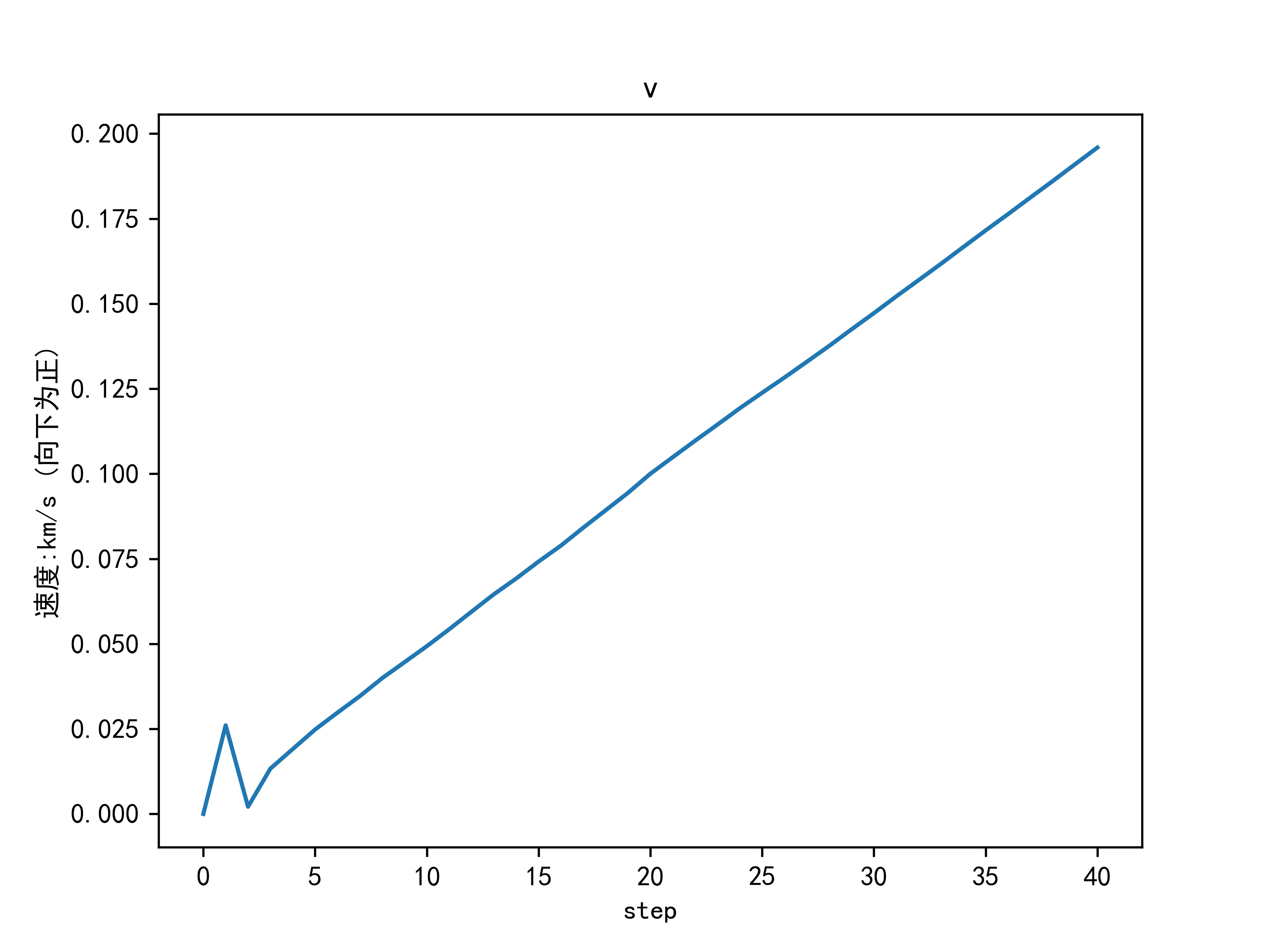
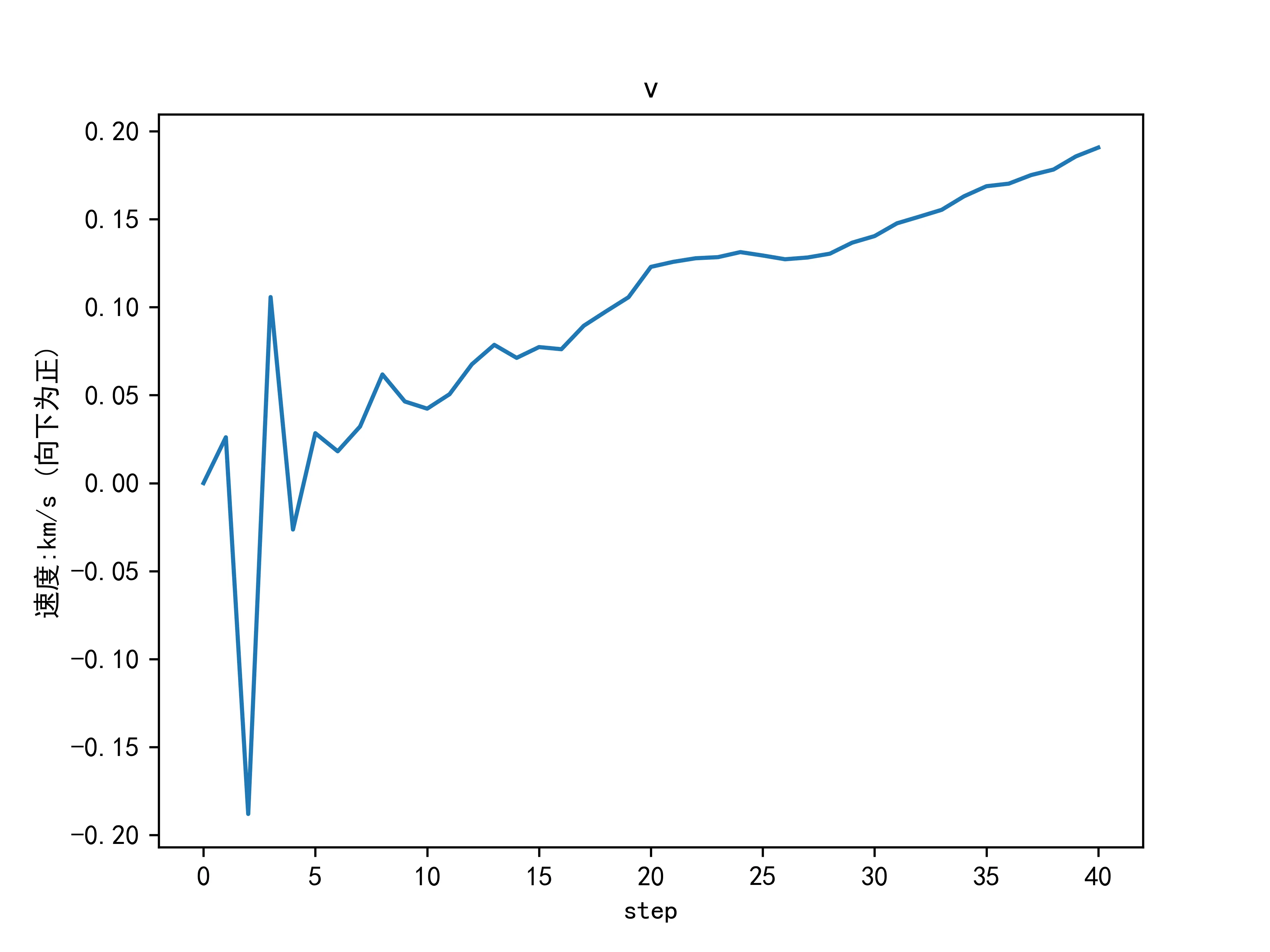
The filtered data of the downward velocity (positive downward) is as follows:
:: | :-: | :-: | :-: | :-: | :-: | :-: | :-: |
Velocity | 0.0078 | 0.0157 | 0.0247 | 0.0343 | 0.0439 | 0.0536 | 0.0635 |
:: | :-: | :-: | :-: | :-: | :-: | :-: | :-: |
Velocity | 0.0733 | 0.0831 | 0.0930 | 0.1028 | 0.1126 | 0.1224 | 0.1322 |
:: | :-: | :-: | :-: | :-: | :-: | :-: | :--: |
Velocity | 0.1420 | 0.1519 | 0.1616 | 0.1714 | 0.1812 | 0.1911 | |
The velocity change graph is shown below:
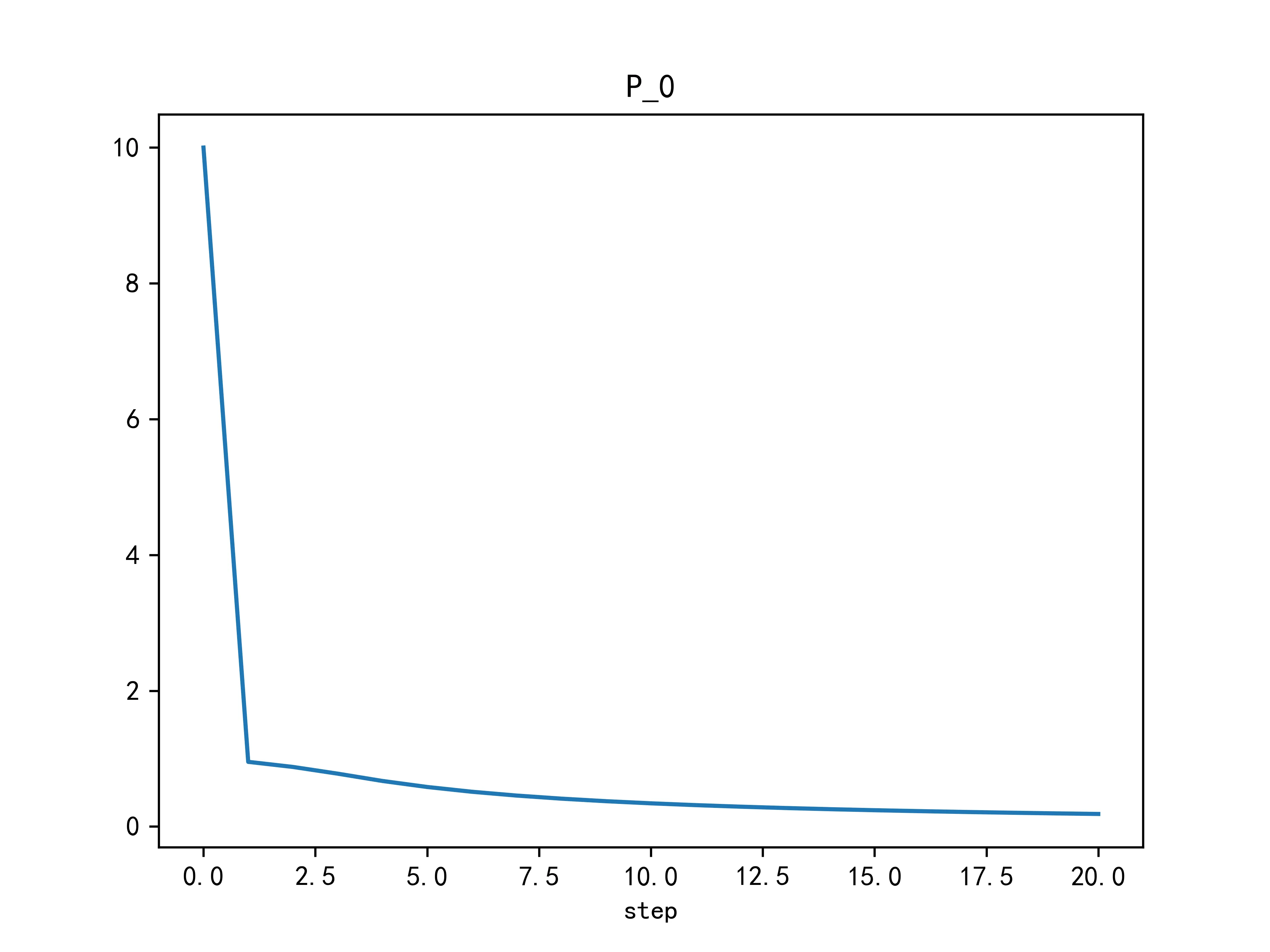
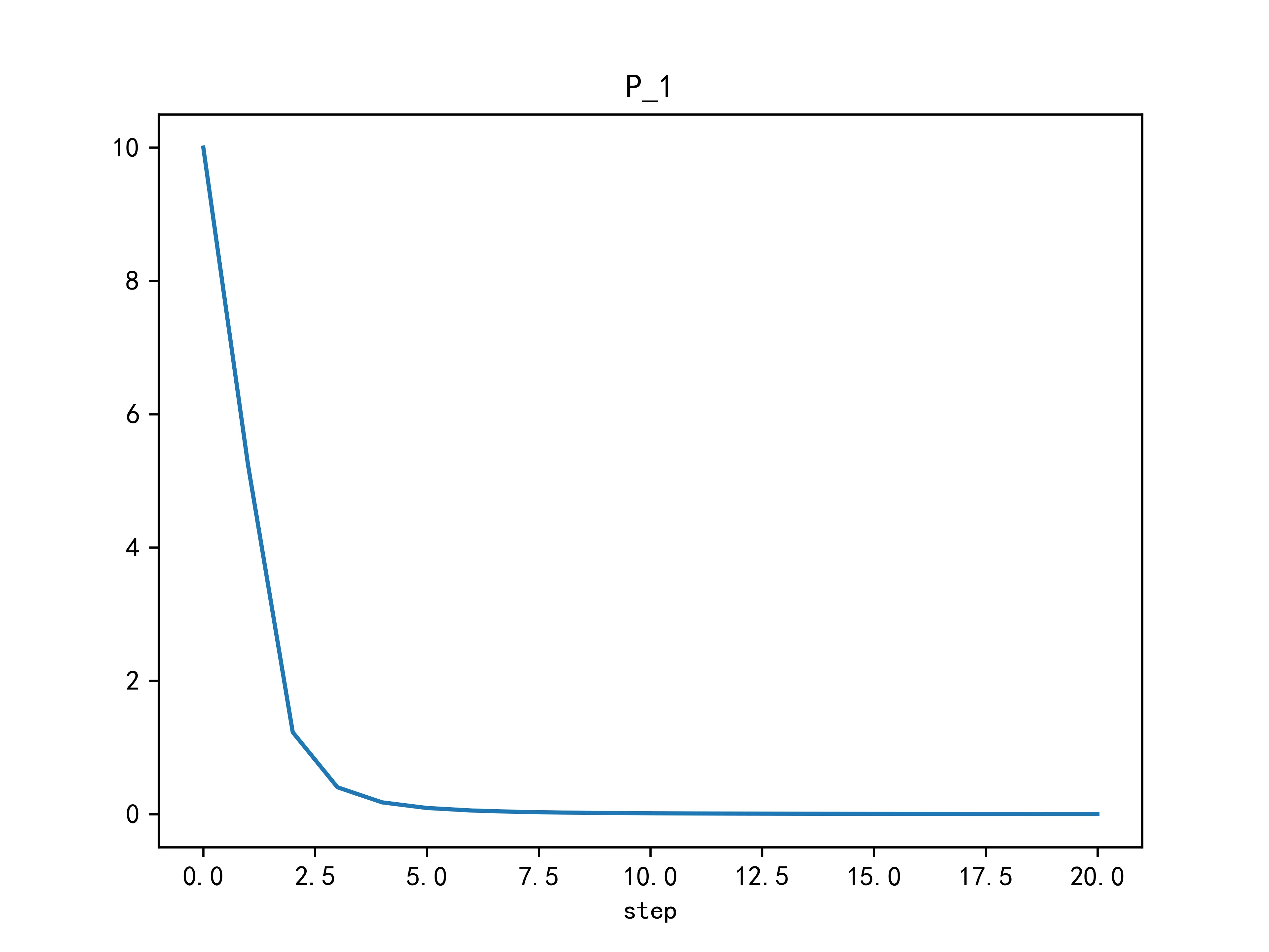
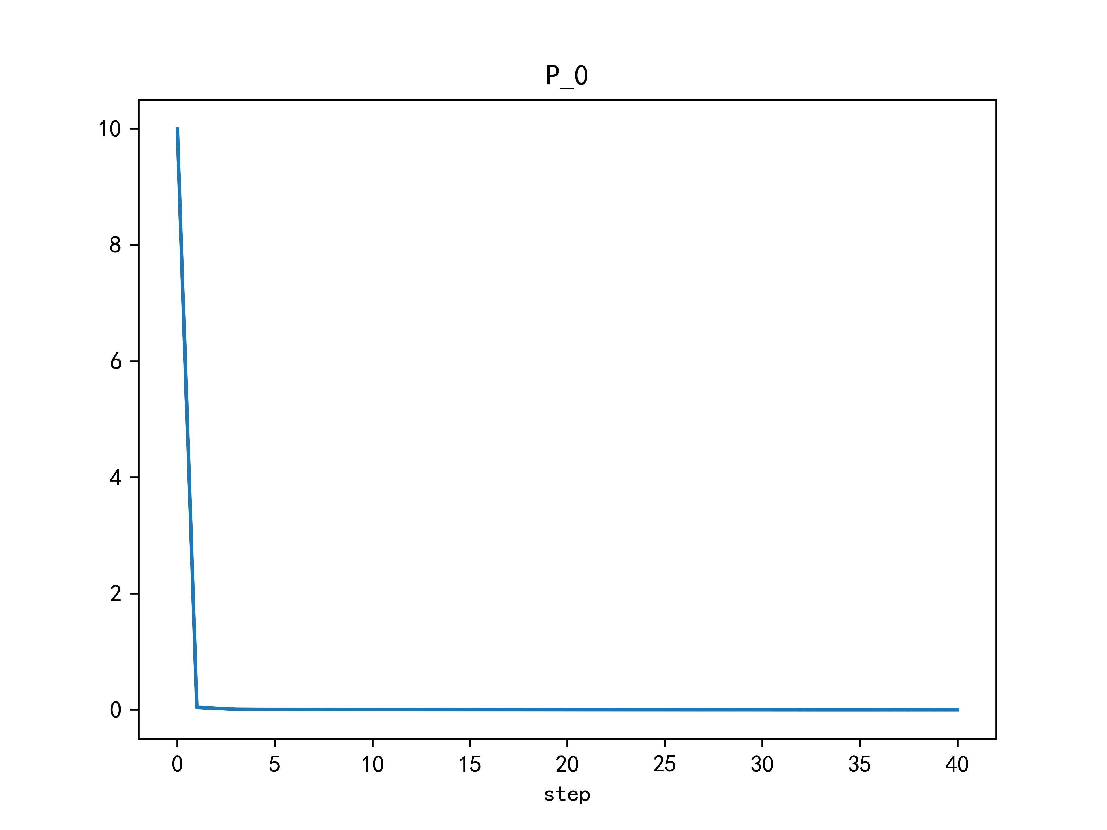
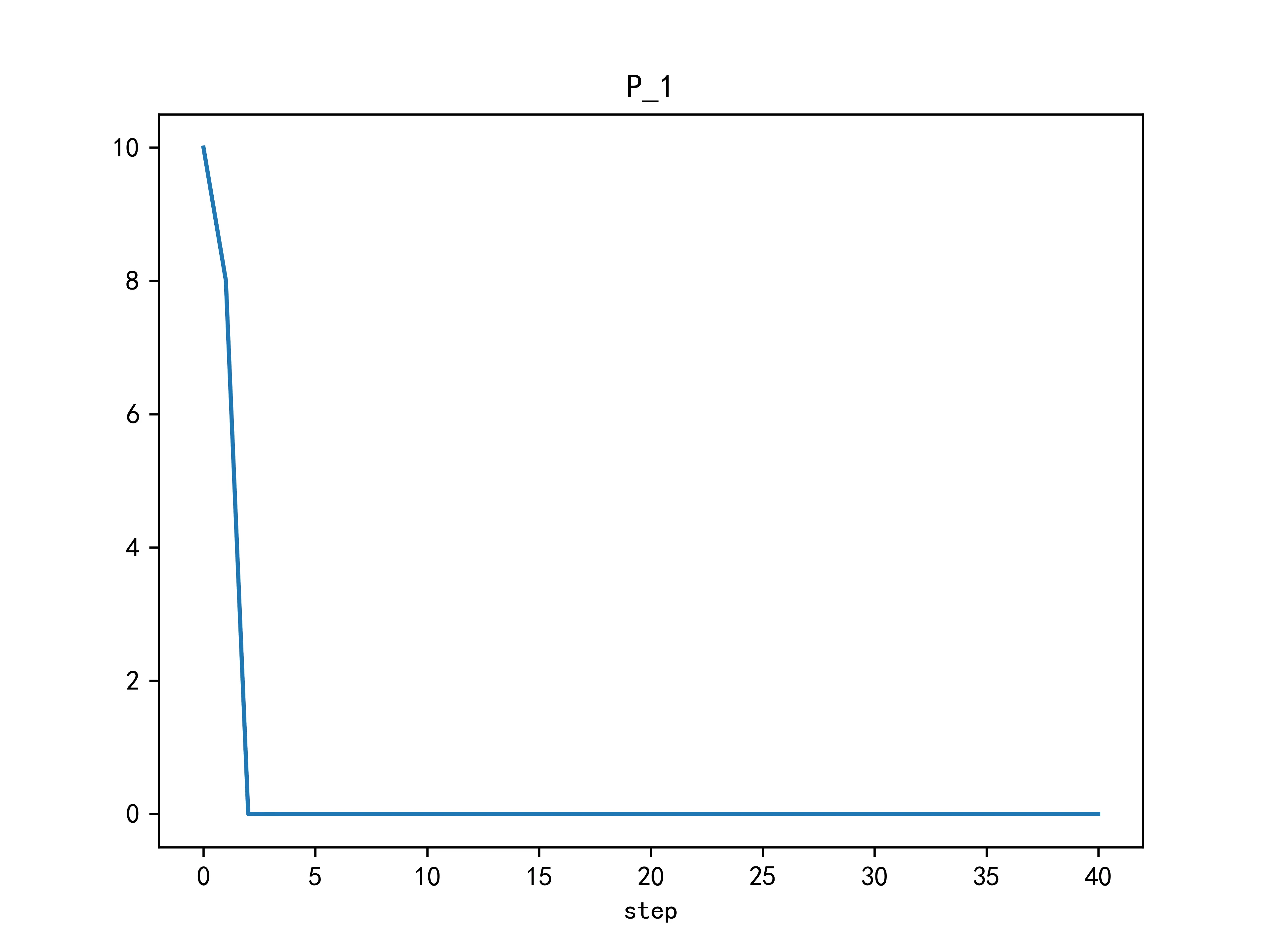
At the same time, the estimated variance of the height and velocity over time is:
|
|
|
|
|
From the above figures, it can be seen that the Kalman filter quickly reduces the estimation of the object's descent height and velocity as soon as the new information is added, and then gradually decreases to near 0 without further significant reduction. The height change curve of the object's free fall is a parabola, and the velocity changes uniformly, which conforms to the relevant physical laws of free fall.
2. Nonlinear Filtering Problem
Based on the given measurement data and the nonlinear filtering model mentioned above, the filtered height and velocity of the falling object are as follows.
The height change is:
The velocity change is:
The estimation error of the object's free fall height and velocity is:
|
|
|
|
|
From the above estimated results, it can be seen that the descent height decreases parabolically with time, and the descent velocity (downward is positive) increases uniformly with time, which conforms to the physical laws of free fall.
Some Findings During the Experiment
In the initial programming and experimental process, since the measurement data given in the problem is in units of \(km\), for ease of calculation, the distance unit is converted to \(km\). However, since the problem does not specify the unit of the measurement variance, the value is not converted and is treated as \(km\).
No anomalies were found during the solution of problem 1. However, when solving problem 2, if the measurement covariance is not converted, and the unit is treated as \(km\), the estimated results will be as shown in the following figure:
|
|
|
|
|
Comparing the calculated results in the above figure with the calculated results in the experimental results of problem 2, it can be seen that the nonlinear Kalman filter is more affected by the measurement error if the measurement covariance is large. This is because the coefficient matrix \(H\) in the nonlinear filter is obtained by local linearization, and if the measurement error itself is large, it will affect the calculation results of the Kalman coefficients, resulting in inaccurate estimation results.
Appendix
Constant Configuration
1 | ''' |
Problem 1 Code
1 | ''' |
Problem 2 Code
```python ''' @ Author: Yu Zhao @ Contact: yuzhaokz@163.com @ Date: 2022-06-17 16:54:31 @ LastEditors: Yu Zhao @ LastEditTime: 2022-06-17 21:02:28 @ Description: 知识因被记录而产生价值 @ Website: https://kezhi.tech '''
import os from pprint import pprint from matplotlib import pyplot as plt import numpy as np
from config import cache_dir,observation_2,param_2
Enable Chinese characters
plt.rcParams['font.sans-serif'] = ['SimHei'] # Used to display Chinese labels normally plt.rcParams['axes.unicode_minus'] = False # Used to display negative signs normally
Create the cache folder
if not os.path.exists(cache_dir): os.mkdir(cache_dir)
Compute H in EKF
def get_H(x): l_2=x[0,0]2+x[2,0]2 return np.matrix( [ [x[0,0]/np.sqrt(l_2),0,x[2,0]/np.sqrt(l_2)], [x[2,0]/l_2,0,-x[0,0]/l_2], ] )
Function of observation
def y(x): return np.matrix( [ [np.sqrt(x[0,0]2+x[2,0]2)], [np.arctan(x[0,0]/x[2,0])], ] )
Kalman filter
def EKF(x_0:np.matrix, # the status of last step P_0:np.matrix, # the variance of last step y_1:np.matrix, # the observation of this step u_0:np.matrix=None, # the input of system Phi:np.matrix=None, # the status transform matrix Psi:np.matrix=None, # coefficient of system input Gamma:np.matrix=None, # coefficient of observing noise R:np.matrix=None, # the variance of observing noise Q:np.matrix=None, # the variance of status noise ): # Check variables if u_0 is None: u_0=np.matrix(0) print("u_0 is missing, use the default value: {}".format(u_0))
if Phi is None:
    Phi=np.matrix(np.eye(x_0.shape[0]))
    print("Phi is missing, use the default value: {}".format(Phi))

if Psi is None:
    Psi=np.matrix(np.zeros((x_0.shape[0],1)))
    print("Psi is missing, use the default value: {}".format(Psi))

if Gamma is None:
    Gamma=np.matrix(np.zeros((x_0.shape[0],1)))
    print("Gamma is missing, use the default value: {}".format(Gamma))

if R is None:
    R=np.matrix(np.zeros((y_1.shape[0],1)))
    print("R is missing, use the default value: {}".format(R))

if Q is None:
    Q=np.matrix(0)
    print("Q is missing, use the default value: {}".format(Q))

# One-step prediction
x_10=Phi@x_0+Psi@u_0
P_10=Phi@P_0@Phi.T+Gamma@Q@Gamma.T
# Local linearization
H=get_H(x_10)
# Time update
P_11=(P_10.I+H.T@R.I@H).I
K_1=P_11@H.T@R.I
x_11=x_10+K_1@(y_1-y(x_10))
return x_11,P_11,K_1
def mse(x_1:np.matrix,x_2:np.matrix): loss=0 for i in range(x_1.shape[0]): for j in range(x_1.shape[1]): loss+=(x_1[i,j]-x_2[i,j])**2 loss=loss/(x_1.shape[0]*x_1.shape[0]) return loss
Iteration EKF, which may have a worse result TAT
def EKF_iter( x_0:np.matrix, # the status of last step P_0:np.matrix, # the variance of last step y_1:np.matrix, # the observation of this step u_0:np.matrix=None, # the input of system Phi:np.matrix=None, # the status transform matrix Psi:np.matrix=None,