Xjtu System Optimization And Scheduling Course Assignments

西安交通大学研究生《系统优化与调度》课程作业

Assignment 1

(1)1.1.2

(a)

$$\begin{gathered} \begin{array}{}\text{(1)}& f(x,y)=(x^2-4{)}^2+y^2 \\ \mathrm{\nabla }f(x,y)=(4x^3-16,2y) \\ {\mathrm{\nabla }}^{2}f(x,y)=\left(\begin{array}{cc}12x^2-16& 0\\ 0& 2\end{array}\right)\end{array} \end{gathered}$$

so there are three stationary points: (2, 0) (-2, 0) and (0, 0)

the Hesse Matrix is positive semi-definite only when $|x|>\frac{4}{3}$

so points (2, 0) (-2, 0) are local minimum points, point (0, 0) is not a local minimum. $$\begin{array}{}\text{(2)}& f(2,0)=f(-2,0)=0\end{array}$$ so (2,0) and (-2,0) are global minimum points of f

let $g(x,y)=-f(x,y)=-(x^2-4{)}^2-y^2$, it is easy to know that Hesse matrix is not positive semi-definite when $x=0,y=0$. So the point(0,0) is not the minimum of $g(x,y)$, which means it is also not the local maximum of $f(x,y)$.

(b)

$$\begin{gathered} \begin{array}{}\text{(3)}& f(x,y)=\frac{1}{2}{x}^2+xcosy \\ \mathrm{\nabla }f(x,y)=(x+cosy,-xsiny)\end{array} \end{gathered}$$

$-xsiny=0$ only if $x=0$ or $y=k\pi (k\in Z)$

if $x=0$, $x+cosy=0$ only if $y=\frac{\pi }{2}+k\pi (k\in Z)$

if $y=k\pi (k\in Z)$, $x+cosy=0$ only if $x=-(-1{)}^k$

so the stationary points of $f(x,y)$ are $(0,\frac{\pi }{2}+k\pi )$ and $(-(-1{)}^k,k\pi )$ $(k\in Z)$ $$\begin{array}{}\text{(4)}& {\mathrm{\nabla }}^{2}f(x,y)=\left(\begin{array}{cc}1& -siny\\ -siny& -xcosy\end{array}\right)\end{array}$$

$$\begin{gathered} \begin{array}{}\text{(5)}& |(1)|>0 \\ |{\mathrm{\nabla }}^{2}f(x,y)|=-xcosy-si{n}^{2}y\end{array} \end{gathered}$$

for points $(0,\frac{\pi }{2}+k\pi )$, $$\begin{array}{}\text{(6)}& |{\mathrm{\nabla }}^{2}f(x,y)|=0-1=-1<0\end{array}$$ for points $(-(-1{)}^k,k\pi )$, $$\begin{array}{}\text{(7)}& |{\mathrm{\nabla }}^{2}f(x,y)|=-1-0=-1<0\end{array}$$ so all the stationary points are not local minimum points.

function $f(x,y)$ have no local minima

(c)

$$\begin{gathered} \begin{array}{}\text{(8)}& f(x,y)=sinx+siny+sin(x+y) \\ \mathrm{\nabla }f(x,y)=(cosx+cos(x+y),cosy+cos(x+y)) \\ {\mathrm{\nabla }}^{2}f(x,y)=\left(\begin{array}{cc}-sinx-sin(x+y)& -sin(x+y)\\ -sin(x+y)& -siny-sin(x+y)\end{array}\right)\end{array} \end{gathered}$$

$$\begin{array}{}\text{(9)}& let\{\begin{array}{lr}cosx+cos(x+y)=0& (1)\\ cosy+cos(x+y)=0& (2)\end{array}\end{array}$$

(1)-(2): $cosx-cosy=0$, so $y=xory=2\pi -x$

if $y=x$, (1) equals to $cosx+cos2x=0$,

using double angle formula: $cosx+2co{s}^{2}x-1=0$

solution: $cosx=\frac{1}{2},-1$, $x=\frac{\pi }{3},\pi ,\frac{5}{3}\pi$

if $y=2\pi -x$, (1) equals to $cosx+1=0$

solution: $cosx=-1$, $x=\pi$

The stationary points are $(\frac{\pi }{3},\frac{\pi }{3}),(\pi ,\pi ),(\frac{5}{3}\pi ,\frac{5}{3}\pi )$. $$\begin{array}{}\text{(10)}& |{\mathrm{\nabla }}^{2}f(x,y)|=sinxsiny+(sinx+siny)sin(x+y)\end{array}$$

for point $(\frac{\pi }{3},\frac{\pi }{3})$: $$\begin{gathered} \begin{array}{}\text{(11)}& |(-sinx-sin(x+y))|=-\sqrt{3} \\ |{\mathrm{\nabla }}^{2}f(x,y)|=\frac{9}{4}\end{array} \end{gathered}$$ its Hesse Matrix is negative definite, so point $(\frac{\pi }{3},\frac{\pi }{3})$ is a local maximum point, max value is $\frac{3}{2}\sqrt{3}$

for point $(\pi ,\pi )$: $$\begin{gathered} \begin{array}{}\text{(12)}& |(-sinx-sin(x+y))|=0 \\ |{\mathrm{\nabla }}^{2}f(x,y)|=0\end{array} \end{gathered}$$ this point is neither a local maximum nor a local minimum.

for point $(\frac{5}{3}\pi ,\frac{5}{3}\pi )$: $$\begin{gathered} \begin{array}{}\text{(13)}& |(-sinx-sin(x+y))|=\sqrt{3} \\ |{\mathrm{\nabla }}^{2}f(x,y)|=-\frac{3}{4}\end{array} \end{gathered}$$ this point is neither a local maximum nor a local minimum.

(d)

$$\begin{gathered} \begin{array}{}\text{(14)}& f(x,y)=(y-x^2{)}^2-x^2 \\ \mathrm{\nabla }f(x,y)=(4x^3-4xy-2x,-2x^2+2y) \\ {\mathrm{\nabla }}^{2}f(x,y)=\left(\begin{array}{cc}12x^2-4y-2& -4x\\ -4x& 2\end{array}\right)\end{array} \end{gathered}$$

$$\begin{array}{}\text{(15)}& let\{\begin{array}{l}4x^3-4xy-2x=0\\ -2x^2+2y=0\end{array}\end{array}$$

Thus the stationary point is $(0,0)$, for this point: $$\begin{gathered} \begin{array}{}\text{(16)}& |(12x^2-4y-2)|=-2 \\ |{\mathrm{\nabla }}^{2}f(x,y)|=-4\end{array} \end{gathered}$$ its Hesse Matrix is neither positive definite nor negative definite, so this stationary point is neither a local maximum nor a local minimum.

(e)

Since the conclusion of (d)——the stationary point is neither a local maximum nor a local minimum, so the minimum point could only exist on the boundary.

Consider $y=-1$, then $f(x,y)=(-1-x^2{)}^2-x^2=x^4+x^2+1$.

In this case, the minimum point is $(0,-1)$ and the minimum is 1

Consider $y=1$, then $f(x,y)=(1-x^2{)}^2-x^2=x^4-3x^2+1$

In this case, the minimum points are $(\frac{\sqrt{6}}{2},1),(-\frac{\sqrt{6}}{2},1)$, and the minimum is $-\frac{5}{4}$.

Summarizing, with the constraint $-1\le y\le 1$ on $y$, there exists global minimum and the global minimum points are $(\frac{\sqrt{6}}{2},1),(-\frac{\sqrt{6}}{2},1)$, the global minimum is $-\frac{5}{4}$.

(2)1.1.6

suppose $x=(a,b),y_i=(a_i,b_i)$, then the problem could transform to: $$\begin{array}{}\text{(17)}& min\sum _{i=1}^m{w}_i\sqrt{(a-a_i{)}^2+(b-b^i{)}^2}\end{array}$$ suppose $f(a,b)=\sum _{i=1}^m{w}_i\sqrt{(a-a_i{)}^2+(b-b^i{)}^2}$, then: $$\begin{gathered} \begin{array}{}\text{(18)}& \mathrm{\nabla }f(x,y)=(\sum _{i=1}^m{w}_i\frac{a-a_i}{\sqrt{(a-a_i{)}^2+(b-b^i{)}^2}},\sum _{i=1}^m{w}_i\frac{b-b_i}{\sqrt{(a-a_i{)}^2+(b-b^i{)}^2}}) \\ {\mathrm{\nabla }}^{2}f(a,b)=\left(\begin{array}{cc}\sum _{i=1}^m{w}_i\frac{2(b-b_i{)}^2}{\sqrt{((a-a_i{)}^2+(b-b^i{)}^2{)}^3}}& \sum _{i=1}^m{w}_i\frac{-2(a-a_i)(b-b_i)}{\sqrt{((a-a_i{)}^2+(b-b^i{)}^2{)}^3}}\\ \sum _{i=1}^m{w}_i\frac{-2(a-a_i)(b-b_i)}{\sqrt{((a-a_i{)}^2+(b-b^i{)}^2{)}^3}}& \sum _{i=1}^m{w}_i\frac{2(a-a_i{)}^2}{\sqrt{((a-a_i{)}^2+(b-b^i{)}^2{)}^3}}\end{array}\right)\end{array} \end{gathered}$$ let $\mathrm{\nabla }f(a,b)=0$, then the stationary point is $(\frac{\sum _{i=1}^m{w}_i{a}_i}{\sum _{i=1}^{m}wi},\frac{\sum _{i=1}^m{w}_i{b}_i}{\sum _{i=1}^{m}wi})$

and ${\mathrm{\nabla }}^{2}f(a,b)$ is positive definite in the point, so it is the global minimum.

(b)

there is only one stationary point in this question, so the solution is unique

(C)

let the plane points on be the reference level

suppose the length of string in weight $i$ is $l_i$, so the problem is: $$\begin{array}{}\text{(19)}& min\sum _{i=1}^m{w}_i(||x-y||-l_i)=\sum _{i=1}^m{w}_i||x-y||-\sum _{i=1}^m{w}_i·l_i\end{array}$$ and we can see that $\sum _{i=1}^m{w}_i·l_i$ is constant, so the problem could transform to: $$\begin{array}{}\text{(20)}& \sum _{i=1}^m{w}_i||x-y||\end{array}$$ which is same as the problem in (a).

(3) 1.2.1

(a)

$$\begin{gathered} \begin{array}{}\text{(21)}& f(x,y)=3x^2+y^4 \\ \mathrm{\nabla }f(x,y)=(6x,4y^3)\end{array} \end{gathered}$$

the start point is $(1,-2)$, so the descend direction is $(-6,32{)}^{\prime }$. Then choose $m$

at first, $m=0,\alpha =s=1$ $$\begin{array}{}\text{(22)}& f(1,2)-f(-5,30)=19-810075=-810056\le -0.1\ast 1\ast -1060=106\end{array}$$

then $m=1，\alpha =\alpha \ast \beta =0.5$ $$\begin{array}{}\text{(23)}& f(1,-2)-f(-2,14)=19-38428=-38409\le -0.1\ast 0.5\ast -1060=53\end{array}$$ then $m=2,\alpha =\alpha \ast \beta =0.25$ $$\begin{array}{}\text{(24)}& f(1,-2)-f(-0.5,6)=19-1296.75=-1277.75\le -0.1\ast 0.25\ast -1060=26.5\end{array}$$ then $m=2,\alpha =\alpha \ast \beta =0.125$ $$\begin{array}{}\text{(25)}& f(1,-2)-f(0.25,2)=19-16.1875\le -0.1\ast 0.125\ast -1060=13.25\end{array}$$ then $m=3,\alpha =\alpha \ast \beta =0.0625$ $$\begin{array}{}\text{(26)}& f(1,-2)-f(0.625,0)=19-1.171875=17.828\ge -0.1\ast 0.0625\ast -1060=6.625\end{array}$$

so the first stepsize is 0.0625, after the iteration, the point changes to $(0.625,0)$

(b)

when $m=0,\alpha =s=1$, the result is above.

then $m=1，\alpha =\alpha \ast \beta =0.1$ $$\begin{array}{}\text{(27)}& f(1,-2)-f(0.4,1.2)=19-2.5536=16.4464\ge -0.1\ast 0.1\ast 1060=-10.6\end{array}$$ so the first stepsize is 0.1, after the iteration, the point changes to $(0.4,1.2)$

(c)

$$\begin{array}{}\text{(28)}& {\mathrm{\nabla }}^{2}f(x,y)=\left(\begin{array}{cc}6& 0\\ 0& 12y^2\end{array}\right)\end{array}$$

at point $(1,-2)$, the Hesse Matrix is: $$\begin{array}{}\text{(29)}& \left(\begin{array}{cc}6& 0\\ 0& 48\end{array}\right)\end{array}$$ its inverse matrix is: $$\begin{array}{}\text{(30)}& \left(\begin{array}{cc}\frac{1}{6}& 0\\ 0& \frac{1}{48}\end{array}\right)\end{array}$$ so the descend direction is: $$\begin{array}{}\text{(31)}& d=-\left(\begin{array}{cc}\frac{1}{6}& 0\\ 0& \frac{1}{48}\end{array}\right)\left(\begin{array}{c}6\\ -32\end{array}\right)=\left(\begin{array}{c}-1\\ \frac{2}{3}\end{array}\right)\end{array}$$ then choose the stepsize:

at first, $m=0,\alpha =s=1$ $$\begin{array}{}\text{(32)}& f(1,-2)-f(0,-\frac{4}{3})=19-3.16=15.84\ge -0.1\ast 1\ast 1060=-106\end{array}$$ so the first stepsize is 1, and the point changes to $(0,-\frac{4}{3})$

Comparing with (a), the computing cost of Newton's method is less

(4) 1.2.6

(a)

PROOF: $$\begin{gathered} \begin{array}{}\text{(33)}& \mathrm{\nabla }f(x)=Qx-b^{\prime } \\ ||\mathrm{\nabla }f(x)-\mathrm{\nabla }f(y)||=||Qx-Qy||\le ||Q||·||x-y||=L·||x-y||\end{array} \end{gathered}$$ (b)

PROOF: $$\begin{gathered} \begin{array}{}\text{(34)}& x^{k+1}=x^k-sD\mathrm{\nabla }f(x^k)=x^k-sD(Q{x}^k-b^{\prime }) \\ {x}^{k+1}=(I-sDQ)x^k+sD{b}^{\prime }\end{array} \end{gathered}$$ ICBS: $$\begin{gathered} \begin{array}{}\text{(35)}& x^{k+1}+C=A(x^k+C) \\ whereA=I-sDQ,B=sD{b}^{\prime },C=(A-I{)}^{-1}B\end{array} \end{gathered}$$ by iteration: $$\begin{gathered} \begin{array}{}\text{(36)}& x^{k+1}+C=A(x^k+C)=A^{k+1}(x^0+C) \\ {x}^{k+1}=A(x^k+C)=A^{k+1}(x^0+C)-C\end{array} \end{gathered}$$ then: $$\begin{gathered} \begin{array}{}\text{(37)}& x^{k+1}=(I-sDQ{)}^{k+1}(x^0-Q^{-1}{b}^{\prime })+Q^{-1}{b}^{\prime } \\ {x}^{k+1}-x^{\ast }=(I-sDQ{)}^{k+1}(x^0-Q^{-1}{b}^{\prime })+Q^{-1}{b}^{\prime }-Q^{-1}{b}^{\prime } \\ {x}^{k+1}-x^{\ast }=(I-sDQ{)}^{k+1}(x^0-Q^{-1}{b}^{\prime }) \\ \end{array} \end{gathered}$$ so: $$\begin{array}{}\text{(38)}& \underset{k\to \mathrm{\infty }}{lim}(x^{k+1}-x^{\ast })=\underset{k\to \mathrm{\infty }}{lim}(I-sDQ{)}^{k+1}(x^0-Q^{-1}{b}^{\prime })\end{array}$$

$$\begin{array}{}\text{(39)}& \mathrm{\forall }s\in (0,2/L),(I-sDQ)<1\end{array}$$

then: $$\begin{gathered} \begin{array}{}\text{(40)}& \underset{k\to \mathrm{\infty }}{lim}(I-sDQ{)}^{k+1}(x^0-Q^{-1}{b}^{\prime })=0 \\ \underset{k\to \mathrm{\infty }}{lim}(x^{k+1}-x^{\ast })=0\end{array} \end{gathered}$$ Summarizing, the method converges to $x^{\ast }=Q^{-1}{b}^{\prime }$ for every starting point $x^0$ if and only if $s\in (0,2/L)$.

(5) 1.3.1

$$\begin{array}{}\text{(41)}& Q=\left(\begin{array}{cc}1& 0.9995\\ 0.9995& 1\end{array}\right)\end{array}$$

$$\begin{gathered} \begin{array}{}\text{(42)}& M=largesteigenvalueofQ=1.9995 \\ m=smallesteigenvalueofQ=0.0005 \\ \frac{f(x^{k+1})}{f(x^k)}\le (\frac{M-m}{M+m}{)}^2=0.999\end{array} \end{gathered}$$

Let $v_m$and $v_M$ be the normalized eigenvectors of Q corresponding

to m and M, respectively, and let $$\begin{array}{}\text{(43)}& x^0=\frac{s}{m}{v}_m\pm \frac{s}{M}{v}_M,s\in R\end{array}$$ Then after the first iteration using the line minimization stepsize

rule,（i.e., a stepsize$\alpha =\frac{2}{M+m}$ ), we get $$\begin{array}{}\text{(44)}& x^1=\frac{M-m}{M+m}(\frac{s}{m}{v}_m\mp \frac{s}{M}{v}_M)=\frac{M-m}{M+m}{x}^0\end{array}$$ Therefore, starting the iterations with$x^0$ , we have for all k $$\begin{array}{}\text{(45)}& \frac{f(x^{k+1})}{f(x^k)}=(\frac{M-m}{M+m}{)}^2\end{array}$$

(6) 1.3.4

$$\begin{gathered} \begin{array}{}\text{(46)}& f(x)=\frac{1}{2}(x-x^{\ast }{)}^{\prime }Q(x-x^{\ast }) \\ \mathrm{\nabla }f(x)=Q(x-x^{\ast })\end{array} \end{gathered}$$

then: $$\begin{gathered} \begin{array}{}\text{(47)}& x^{k+1}=x^k-s(Q(x^k-x^{\ast })+e^k) \\ {x}^{k+1}=x^k(I-sQ)+sQ{x}^{\ast }+s{e}^k \\ {x}^{k+1}-x^{\ast }=(x^k-x^{\ast })(I-sQ)+s{e}^k\end{array} \end{gathered}$$ since for any $AB,||A·B||\le ||A||·||B||$ $$\begin{array}{}\text{(48)}& ||x^{k+1}-x^{\ast }||\le ||(x^k-x^{\ast })(I-sQ)||+s||e^k||\end{array}$$ then: $$\begin{array}{}\text{(49)}& ||x^{k+1}-x^{\ast }||\le ||x^k-x^{\ast }||·q+s\delta \end{array}$$ by the iteration, $$\begin{array}{}\text{(50)}& ||x^k-x^0||\le q^k||x0-x^k||+s\delta (1+q+q^2+...+q^{k-1})\end{array}$$ so: $$\begin{array}{}\text{(51)}& ||x^k-x^0||\le q^k||x0-x^k||+\frac{s\delta }{1-q}\end{array}$$ i.e. $$\begin{array}{}\text{(52)}& ||x^k-x^0||\le \frac{s\delta }{1-q}+q^k||x0-x^k||\end{array}$$

(7) 1.4.1

In Newton's Method, we have: $$\begin{array}{}\text{(53)}& x^{k+1}=x^k-{\alpha }^k({\mathrm{\nabla }}^{2}f(x^k){)}^{-1}\mathrm{\nabla }f(x^k)\end{array}$$ consider $x=Sy$, then: $$\begin{gathered} \begin{array}{}\text{(54)}& S{y}^{k+1}=S{y}^k-S^{-2}{\alpha }^k({\mathrm{\nabla }}^{2}f(S{y}^k){)}^{-1}S\mathrm{\nabla }f(S{y}^k) \\ {y}^{k+1}=y^k-S^{-1}{\alpha }^k({\mathrm{\nabla }}^{2}f(S{y}^k){)}^{-1}\mathrm{\nabla }f(S{y}^k)\end{array} \end{gathered}$$ since $y=S^{-1}x$, consider $y^0=S^{-1}{x}^0$, then: $$\begin{gathered} \begin{array}{}\text{(55)}& y^1=y^0-S^{-1}{\alpha }^0({\mathrm{\nabla }}^{2}f(S{y}^0){)}^{-1}\mathrm{\nabla }f(S{y}^0) \\ {y}^1=S^{-1}{x}^0-S^{-1}{\alpha }^0({\mathrm{\nabla }}^{2}f(x^0){)}^{-1}\mathrm{\nabla }f(x^0)\end{array} \end{gathered}$$ so $y^1=S^{-1}{x}^1$, for $y^k=S^{-1}{x}^k$: $$\begin{gathered} \begin{array}{}\text{(56)}& y^{k+1}=y^k-S^{-1}{\alpha }^k({\mathrm{\nabla }}^{2}f(S{y}^k){)}^{-1}\mathrm{\nabla }f(S{y}^k) \\ {y}^{k+1}=S^{-1}{x}^k-S^{-1}{\alpha }^k({\mathrm{\nabla }}^{2}f(S{y}^k){)}^{-1}\mathrm{\nabla }f(S{y}^k) \\ {y}^{k+1}=S^{-1}{x}^{k+1}\end{array} \end{gathered}$$ summarizing, the sequence made by Newton's Method $y^k=S^{-1}{x}^k$.

## (8)

PROOF:

Since $f(x)$ is convex, $$\begin{array}{}\text{(57)}& \mathrm{\forall }{x}_1,x_2\in \mathrm{\Omega },\lambda \in (0,1)\lambda f(x_1)+(1-\lambda )f(x_2)\ge f(\lambda x_1+(1-\lambda )x_2)\end{array}$$ Since $\gamma (x)$ is a monotone nondecreasing function, $$\begin{array}{}\text{(58)}& \gamma (\lambda f(x_1)+(1-\lambda )f(x_2))\ge \gamma (f(\lambda x_1+(1-\lambda )x_2))\end{array}$$ Since $\gamma (x)$ is convex, $$\begin{array}{}\text{(59)}& \lambda \gamma (f(x_1))+(1-\lambda )\gamma (f(x_2))\ge \gamma (\lambda f(x_1)+(1-\lambda )f(x_2))\end{array}$$ Therefore, $$\begin{array}{}\text{(60)}& \lambda \gamma (f(x_1))+(1-\lambda )\gamma (f(x_2))\ge \gamma (f(\lambda x_1+(1-\lambda )x_2))\end{array}$$ This implies that $\gamma (f)(x)$ is convex.

(9)

(a)

$$\begin{gathered} \begin{array}{}\text{(61)}& f(x,y)=5x^2+5y^2-xy-11x+11y+11 \\ \mathrm{\nabla }f(x,y)=(10x-y-11,10y-x+11)\end{array} \end{gathered}$$

$$\begin{array}{}\text{(62)}& let\{\begin{array}{l}10x-y-11=0\\ 10y-x+11=0\end{array}\end{array}$$

the solution of the equation set above is $(1,-1)$,

it is the point satisfying the first-order necessary conditions

(b)

$$\begin{array}{}\text{(63)}& {\mathrm{\nabla }}^{2}f(x,y)=\left(\begin{array}{cc}10& -1\\ -1& 10\end{array}\right)\end{array}$$

it is easy to know the Hessian Matrix is always positive definite, so the point$(1,-1)$ is a global minimum point, and the global minimum is 0

(c)

for the steepest decent method, $D^k=I$ $$\begin{array}{}\text{(64)}& (D^k{)}^{\frac{1}{2}}{\mathrm{\nabla }}^{2}f(x,y)(D^k{)}^{\frac{1}{2}}={\mathrm{\nabla }}^{2}f(x,y)=\left(\begin{array}{cc}10& -1\\ -1& 10\end{array}\right)\end{array}$$

$$\begin{gathered} \begin{array}{}\text{(65)}& M=11,m=9 \\ \frac{f(x^{k+1})-f(x^{\ast })}{f(x^k)-f(x^{\ast })}\le (\frac{M-m}{M+m}{)}^2=0.01\end{array} \end{gathered}$$

(10)

(a)

$$\begin{gathered} \begin{array}{}\text{(66)}& f(x,y)=x^2+y^2+xy-3x \\ \mathrm{\nabla }f(x,y)=(2x+y-3,x+2y) \\ {\mathrm{\nabla }}^{2}f(x,y)=\left(\begin{array}{cc}2& 1\\ 1& 2\end{array}\right)\end{array} \end{gathered}$$

$$\begin{array}{}\text{(67)}& let\{\begin{array}{l}2x+y-3=0\\ x+2y=0\end{array}\end{array}$$

the solution of the equation set above is $(2,-1)$, and the Hessian Matrix is always positive definite,

so point $(2,-1)$ is unconstrained local minimum point.

(b)

Because Hessian Matrix is always positive definite, the function $f(x,y)$ is convex for all point in the real space.

(c)

the minimum points must on the boundary of the constraint.

consider $x=0$, then $f(x,y)=y^2$, the minimum point is $(0,0)$ and the minimum is $0$

consider $y=0$, then $f(x,y)=x^2-3x$, the minimum point is $(\frac{3}{2},0)$ and the minimum is $-\frac{9}{4}$

therefore, the minimum point of f subject to $x\ge 0,y\ge 0$ is $(\frac{3}{2},0)$ and the minimum is $-\frac{9}{4}$

(d)

for the steepest decent method, $D^k=I$ $$\begin{array}{}\text{(68)}& (D^k{)}^{\frac{1}{2}}{\mathrm{\nabla }}^{2}f(x,y)(D^k{)}^{\frac{1}{2}}={\mathrm{\nabla }}^{2}f(x,y)=\left(\begin{array}{cc}2& 1\\ 1& 2\end{array}\right)\end{array}$$

$$\begin{gathered} \begin{array}{}\text{(69)}& M=3,m=1 \\ \frac{f(x^{k+1})-f(x^{\ast })}{f(x^k)-f(x^{\ast })}\le (\frac{M-m}{M+m}{)}^2=\frac{1}{4}\end{array} \end{gathered}$$

Assignment 2

(1)

Q: Consider the quadratic program $$\begin{gathered} \begin{array}{}\text{(70)}& min0.5x^{T}Qx-b^{T}x \\ s.t.Ax=c\end{array} \end{gathered}$$ Prove that $x^{\ast }$ is a local minimum point if and only if it is a global minimum point.(No convexity is assumed)

Proof:

Since no convexity is assumed, we consider two cases:

1. If Q is a positive definitive matrix. It’s obvious that $x^{\ast }$ is a local minimum point if and only if it is a global minimum point.

2. If Q is not a positive definitive matrix.

Assume $x^{\ast }$ is a local minimum point, set $x^{\ast }+d$ as the global minimum point.

so $A(x^{\ast }+d)=c$

and because $A(x^{\ast })=c$

so $Ad=0$

so we have $A(x\ast +2d)=c$

then according to the optimality condition, we have $$\begin{gathered} \begin{array}{}\text{(71)}& \mathrm{\nabla }f(x^{\ast }+d{)}^{\prime }((x^{\ast }+2d)-(x^{\ast }+d))\ge 0 \\ (Q(x^{\ast }+d)-b^{\prime })d\ge 0\end{array} \end{gathered}$$ and we have $$\begin{array}{}\text{(72)}& f(x^{\ast }+d)& =0.5(x^{\ast }+d{)}^{\prime }Q(x^{\ast }+d)-b^{\prime }(x^{\ast }+d)\text{(73)}& & =0.5x^{{\ast }^{\prime }}Q{x}^{\ast }-b{x}^{\ast }+(Q(x^{\ast }+d)-b^{\prime })d-0.5d^{\prime }Qd\text{(74)}& & =f(x^{\ast })+(Q(x^{\ast }+d)-b^{\prime })d-0.5d^{\prime }Qd\end{array}$$ as $(Q(x^{\ast }+d)-b^{\prime })d\ge 0$ and $-0.5d^{\prime }Qd\ge 0$

then $f(x^{\ast }+d)\ge f(x^{\ast })$

and because $f(x^{\ast }+d)$ is the global minimum, so we can get that $f(x^{\ast }+d)=f(x^{\ast })$. and then we can conclude that the local minimum is the global minimum.

(2)

Suppose that the projected negative nablaient d is calculated satisfying $$\begin{array}{}\text{(75)}& -g=d+A_q^T\lambda \end{array}$$ and that some component ${\lambda }_i$ of $\lambda$, corresponding to an inequality, is negative. Show that if the $i$th inequality is dropped, the projection $d_i$ of the negative nablaient onto the remaining constraints is a feasible direction of decent

Proof:

Let the new direction vector $d_i$ by relaxing the $i$th constraint and projecting the negative nablaient onto the subspace determined by remaining $q-1$ active constraints.

Let $A_{\overline{q}}$ denote the matrix $A_q$ with row $a_j$ deleted.

We know that $g^T{d}_i<0$ .

Multiplying the equation $-g=d_i+A_{\overline{q}}^T{\lambda }_i$ by $d_i$ and using $A_{\overline{q}}{d}_i=0$ we obtain: $$\begin{array}{}\text{(76)}& 0>g^T{d}_i=-{\lambda }_i{a}_i^T{d}_i\end{array}$$ Since ${\lambda }_i<0$ , we conclude that $d_i^T{d}_i<0$ .

So the vector $d_i$ is a direction of descent, but it is a feasible direction.

(3) 3.1.9

(a)

$$\begin{gathered} \begin{array}{}\text{(77)}& minx+y+z \\ s.t.xyz={\rho }^2(x+y+z)\end{array} \end{gathered}$$

consider the Lagrangian Relaxation: $$\begin{array}{}\text{(78)}& L(x,y,z,\lambda )=x+y+z+\lambda (xyz-{\rho }^2(x+y+z))\end{array}$$ let $\mathrm{\nabla }L=0$, then we have $$\begin{array}{}\text{(79)}& \{\begin{array}{l}1+\lambda (yz-{\rho }^2)=0\\ 1+\lambda (xz-{\rho }^2)=0\\ 1+\lambda (xy-{\rho }^2)=0\\ xyz={\rho }^2(x+y+z)\end{array}\end{array}$$ then we have: $$\begin{array}{}\text{(80)}& \frac{y+z}{x}=\frac{x+z}{y}=\frac{x+y}{z}\end{array}$$ so $x=y=z$

(b)

consider all lines parallel to the line that passes through $a$ and $b$ and

intersect the circle.

the maximal area appears only if the point $x$ is the point of tangency between the parallel line and the circle.

and we can see that the line through $x$ and $\hat{x}$ is also the line perpendicular to the tangent line and through point $x$.

so this line must passes through the center of the circle.

(c)

Fix two vertices and the corresponding side of the corresponding side of the triangle and optimize vertex and the vertex of the circle should be orthogonal to the fixed side. Hence, the optimal is obtained when the two remaining side are equal. Repeating this argument, fixing each side of the triangle in turn, we see that all sides should be equal.

(d)

Similar line of argument as in (c).

(4) 3.3.5

(a)

Let $d\in \overline{F}(x^{\ast })$, so $\mathrm{\exists }\{d^k\}\subset F(x^{\ast })$, so that $d^k\to d$.

And we have: $$\begin{array}{}\text{(81)}& \mathrm{\nabla }f(x^{\ast }{)}^{\prime }{d}^k=li{m}_{\alpha \to 0}\frac{f(x^{\ast }+\alpha d^k)-f(x^{\ast })}{\alpha }\end{array}$$

Because $x^{\ast }$ is a constrained local minimum, so$\frac{f(x^{\ast }+\alpha d^k)-f(x^{\ast })}{\alpha }\ge 0$ .

So, $\mathrm{\nabla }f(x^{\ast }{)}^{\prime }{d}^k\ge 0$.

(b)

If x* is a constrained local minimum, from (a) we can get $$\begin{array}{}\text{(82)}& \mathrm{\nabla }f(x^{\ast }{)}^{\prime }{d}^k\ge 0,\mathrm{\forall }dwith\mathrm{\nabla }{g}_j(x^{\ast }{)}^{\prime }d\le 0,\mathrm{\forall }j\in A(x^{\ast })\end{array}$$ According to Farkas’Lemma, it is true iff there exists $u^{\ast }$ such that $$\begin{array}{}\text{(83)}& -\mathrm{\nabla }f(x^{\ast })=\sum _{j\in A(x^{\ast })}{u}_j\mathrm{\nabla }{g}_j(x^{\ast }),u_j^{\ast }\ge 0\end{array}$$ Setting $u_j^{\ast }=0$ for $j\notin A(x^{\ast })$ .

we have the desired result.

(c)

We want to show that $\overline{F}(x^{\ast })=V(x)$, where $V(x^{\ast })$ is the cone of first order feasible variations given by $V(x^{\ast })=\{d|\mathrm{\nabla }{g}_j(x^{\ast }{)}^{\prime }d\le 0,\mathrm{\forall }j\in A(x^{\ast }\}$.

From Mean Value Theorem, for each $j\in A(x^{\ast })$ and for any $d\in F(x^{\ast })$ there exist $\epsilon \in [0,1]$ such that $g_j(x^{\ast }+\alpha d)=g_j(x^{\ast })+\alpha \mathrm{\nabla }{g}_j(x^{\ast }+\epsilon \alpha d{)}^{\prime }d$.

Because $g_j(x^{\ast }+\alpha d)\le 0$, so $$\begin{array}{}\text{(84)}& \underset{\alpha \to 0}{lim}\alpha \mathrm{\nabla }{g}_j(x^{\ast }+\epsilon \alpha d{)}^{\prime }d\le 0\end{array}$$ And that implies that $g_j(x^)d,jA(x^ $, so that $d\in V(x^{\ast })$. Therefore $F(x^{\ast })\subset V(x)$, since $V(x^{\ast })$ is closed, so $\overline{F}(x^{\ast })\subset V(x)$.

From each of 1-4, we can also prove that $\overline{F}(x^{\ast })\supset V(x)$.

So we can get that $F(x^{\ast })=V(x)$.

(d)

We can easily get the local minimum is $x^{\ast }=(0,0)$. So we have $$\begin{gathered} \begin{array}{}\text{(85)}& \mathrm{\nabla }{g}_1(0,0)=(0,1{)}^T \\ \mathrm{\nabla }{g}_2(0,0)=(0,-1{)}^T\end{array} \end{gathered}$$ Obviously g1 and g2 are not linear, so the condition(1) is violated. Furthermore, there is no vector $d=(d1,d2{)}^{\prime }$ such that $$\begin{array}{}\text{(86)}& \mathrm{\nabla }{g}_1(0,0{)}^{\prime }d=d_2<0,\mathrm{\nabla }{g}_1(0,0{)}^{\prime }d=-d_2<0\end{array}$$

So the condition2 is violated. Similarly, condition3 is violated. The vectors $\mathrm{\nabla }{g}_1(0,0)$ and $\mathrm{\nabla }{g}_2(0,0)$ are linearly dependent since $\mathrm{\nabla }{g}_1(0,0)=-\mathrm{\nabla }{g}_2(0,0)$, so the condition4 is violated.

Assume $u_0\mathrm{\nabla }f(x^{\ast })+u_1\mathrm{\nabla }{g}_1(x^{\ast })+u_2\mathrm{\nabla }{g}_2(x^{\ast })=0$, so we have: $$\begin{array}{}\text{(87)}& (u_0,u_0{)}^{\prime }+(0,u_1{)}^{\prime }+(0,u_2{)}^{\prime }=(0,0{)}^{\prime }\end{array}$$ It follows that $u_0=0$. So there is no Lagrange multiplier.

(e)

From the description we know that $x^{\ast }$ is also a local minimum for the modified problem.

The modified problem has a single constraint $g_1(x)=||h(x)|{|}^2$, which is active at $x^{\ast }$.

Since $g_1$ is not linear, the condition 1 is violated.

Because $\mathrm{\nabla }{g}_1(x^{\ast })=2\mathrm{\nabla }h(x^{\ast })\mathrm{\nabla }h(x^{\ast })=0$, the conditions 2 and 4 are violated. If condition 3 holds, we can prove that condition 2 is hold too, so condition 3 is violated, too. From $u_0^{\ast }\mathrm{\nabla }g(x^{\ast }=-u_1^{\ast }\mathrm{\nabla }{g}_1(x^{\ast }))$ and $\mathrm{\nabla }{g}_1(x^{\ast })=0$, it follows that $u_0^{\ast }=0$, so there is no Lagrange multiplier.

(5) 5.1.7

(a)

$$\begin{array}{}\text{(88)}& let{x}_i=\{\begin{array}{lr}0& iftheobjectisincludedinthesubset\\ 1& otherwise\end{array}\end{array}$$

Then the total weight and value of objects included is $\sum _i{w}_i{x}_i$ and iv_ix_i, respectively, and the problem can be written as $$ max f(x)={i=1}^nv_ix_i\

19. t._{i=1}^nw_ix_iA, xi ∈ {0, 1}, i= 1, . . . , n. $$

(b)

Let $\hat{f}(x)=-f(x)$ and consider the equivalent problem of minimizing $\hat{f}(x)$ subject to the constraints given above. Then $$\begin{array}{}\text{(89)}& L(x,\mu )=-\sum _{i=1}^n{v}_i{x}_i+\mu (\sum _{i=1}^n{w}_i{x}_i-A)\end{array}$$ and $$\begin{array}{}\text{(90)}& \hat{q}(u)=\underset{x_i\in \{0,1\}}{inf}\{\sum _{i=1}^n(\mu w_i-v_i)x_i-\mu A\}\end{array}$$ Note that the minimization above is a separable problem, and the minimum is attained at $$\begin{array}{}\text{(91)}& {\hat{x}}_i(\mu )=\{\begin{array}{lr}0& if\mu <v_i/w_i\\ 1& if\mu >v_i/w_i\\ oor1& otherwise\end{array}\end{array}$$ Without loss of generality, assume that the objects are ordered such that: $$\begin{array}{}\text{(92)}& \frac{v_1}{w_1}\le \frac{v_2}{w_2}\le ...\le \frac{v_n}{w_n}\end{array}$$ When$\mu \in (\frac{v_{j-1}}{w_{j-1}},\frac{v_j}{w_j}]$ for some $j$ with $1\le j\le n$, then ${\hat{x}}_i=1$ for all $i\ge j$.

And $x_i()=0$ otherwise, and $$\begin{array}{}\text{(93)}& \hat{q}(\mu )=u(\sum _{i=1}^n{w}_i-A)-\sum _{i=1}^n{v}_i\end{array}$$ From this relation, we see that, as μ increases, the slope of $\hat{q}(u)$ decreases from $\sum _{i=1}^n{w}_i-A$ to $-A$. Therefore, if ${}_{i=1}^n{w}_i-A>0$, $\hat{q}(u)$ is maximized when the slope of the curve goes from positive to negative. In this case, the dual optimal value ${\hat{q}}^{\ast }$ is attained at $u^{\ast }=\frac{v_i^{\ast }}{w_i^{\ast }}$, where$i^{\ast }$is the largest $i$ such that $$\begin{array}{}\text{(94)}& w_1+w_2+...+w_n\ge A\end{array}$$

If $\sum _{i=1}^n{w}_i-A\le 0$, then the dual optimal value ${\hat{q}}^{\ast }$is attained at $u^{\ast }=0$.

(c)

Consider a relaxed version of the problem of minimizing $\hat{f}$: $$ max f_R(x)=-_{i=1}^nv_ix_i\

19. t._{i=1}^nw_ix_iA, xi ∈ [0, 1], i= 1, . . . , n. $$ Let $f_R^{\ast }$ and $q_R^{\ast }$ be the optimal values of the relaxed problem and its dual, respectively.

In the relaxed problem, the cost function is convex over $R^n$(in fact it is linear), and the constraint set is polyhedral.

Thus, according to Prop. 5.2.1, there is no duality gap, and $f_R^{\ast }=q_R^{\ast }$ . The dual function of the relaxed problem is: $$\begin{array}{}\text{(95)}& q_R(\mu )=\underset{x_i\in \{0,1\}}{inf}\{\sum _{i=1}^n(\mu w_i-v_i)x_i-\mu A\}\end{array}$$

Again, $q_R(x)$is separable and the minimum is attained at $$\begin{array}{}\text{(96)}& {\hat{x}}_i(\mu )=\{\begin{array}{lr}0& if\mu <v_i/w_i\\ 1& if\mu >v_i/w_i\\ oor1& otherwise\end{array}\end{array}$$ Thus the solution is the same as the $\{0,1\}$ constrained problem for all $i$ with $\mu \ne \frac{v_i}{w_i}$. For $i$ with$\mu =\frac{v_i}{w_i}$, the value of $x_i$ is irrelevant to the dual function value. Therefore, $\hat{q}(u)=q_R(\mu )$ for all μ, and thus ${\hat{q}}^{\ast }=q_R^{\ast }$.

Following Example 5.1.2, it can be seen that the optimal primal and dual solution pair $(x^{\ast },{\mu }^{\ast })$ of the relaxed problem satisfies $$ μ∗ w_i = v_i ,  if 0 <x_i^*< 1,\

μ∗ w_i v_i ,  if x_i^*=0,\

μ∗ w_i v_i ,  if x_i^*= 1, $$

In fact, it is straightforward to show that there is an optimal solution of the relaxed problem such that at most one $x_i^{\ast }$ satisfies $0<x_i^{\ast }<1$. Consider a solution equivalent to this optimal solution with the exception that = 0 if 0 < < 1. This solution is clearly feasible for the {0, 1} constrained problem, so that we have $$\begin{array}{}\text{(97)}& {\hat{f}}^{\ast }\le \hat{f}(\hat{x})\le f_R^{\ast }+\underset{i\le i\le n}{max}{v}_i\end{array}$$ Combining with earlier results, $$\begin{array}{}\text{(98)}& {\hat{f}}^{\ast }\le q_R^{\ast }+\underset{i\le i\le n}{max}{v}_i={\hat{q}}^{\ast }+\underset{i\le i\le n}{max}{v}_i\end{array}$$ Since ${\hat{f}}^{\ast }=-f$ and ${\hat{q}}^{\ast }=-q^{\ast }$ we have the desired result.

(d)

Since the object weights and values remain the same we have from (c) that $0\le q^{\ast }(k)-f^{\ast }(k)\le \underset{i\le i\le n}{max}{v}_i$. By including in the subset each replica of an object assembled in the optimal solution to the original problem, we see that $f^{\ast }(k)\ge k{f}^{\ast }$ . It then follows that $$\begin{array}{}\text{(99)}& \underset{k\to \mathrm{\infty }}{lim}(q^{\ast }(k)-f^{\ast }(k))=0\end{array}$$

Assignment 3

5.5.2

$$\begin{gathered} \begin{array}{}\text{(100)}& minf(x)=10x_1+3x_2 \\ s.t.5x_1+x_2\ge 4x_1,x_2\in \{0,1\}\end{array} \end{gathered}$$

Using Lagrangian relaxiation:

the Lagrangian funcion is $$\begin{array}{}\text{(101)}& L(x,\mu )=10x_1+3x_2+\mu (4-5x_1-x_2)=(10-5\mu )x_1+(3-\mu )x_2+4\mu \end{array}$$ the dual problem is: $$\begin{gathered} \begin{array}{}\text{(102)}& maxq(\mu )=\underset{x\in \{0,1\}}{min}L(x,\mu ) \\ s.t.\mu \ge 0\end{array} \end{gathered}$$ the solution is $\mu =2,q^{\ast }=8$

Using constraint relaxation:

the releaxed problem is: $$\begin{gathered} \begin{array}{}\text{(103)}& minf(x)=10x_1+3x_2 \\ s.t.5x_1+x_2\ge 4x_1,x_2\in [0,1]\end{array} \end{gathered}$$ (a) when $x_1=0$, the prolem is: $$\begin{gathered} \begin{array}{}\text{(104)}& minf(x)=3x_2 \\ s.t.x_2\ge 4x_2\in [0,1]\end{array} \end{gathered}$$ this problem is infeasible.

2. when $x_1=1$, the problem is: $$\begin{gathered} \begin{array}{}\text{(105)}& minf(x)=10+3x_2 \\ s.t.5+x_2\ge 4x_2\in [0,1]\end{array} \end{gathered}$$ when $x_2=0$, the value of object function is minimization. so the solution is $(1,0)$, it is also integer solution, so the point $(1,0)$ is the optimal point of the primal problem, minimization is 10

so the lower bound of Lagrangian relaxiation is less than constraint relaxation.

5.5.10

1. $$\begin{gathered} \begin{array}{rl}\overline{q}& =\underset{x\in \overline{X}}{inf}\{f(x)+\sum _{j=0}^{\overline{r}}{\mu }_j{g}_j(x)\}\\ & =\underset{x\in X \\ {g}_{\overline{r}+1}(x)\le 0...g_r(x)\le 0}{inf}\{f(x)+\sum _{j=1}^{\overline{r}}{\mu }_j{g}_j(x)\}\\ & \ge \underset{x\in X \\ {g}_{\overline{r}+1}(x)\le 0...g_r(x)\le 0}{inf}\{f(x)+\sum _{j=1}^r{\mu }_j{g}_j(x)\}\\ & \ge \underset{x\in X}{inf}\{f(x)+\sum _{j=1}^r{\mu }_j{g}_j(x)\}\\ & =q\end{array} \end{gathered}$$ so we have ${\overline{q}}^{\ast }\ge q^{\ast }$, and we have ${\overline{q}}^{\ast }\le f^{\ast }$ by the weak duality theorem, so $q^{\ast }\le {\overline{q}}^{\ast }\le f^{\ast }$

if $q^{\ast }=f^{\ast }$, and we have$q^{\ast }\le {\overline{q}}^{\ast }\le f^{\ast }$

so we can get $q^{\ast }={\overline{q}}^{\ast }=f^{\ast }$

3. $$\begin{gathered} \begin{array}{}\text{(106)}& minf(x)=e^{-x_1{x}_2} \\ s.t.x_1=0,x_1-1\le 0,x\in X=\{x|x\ge 0\}\end{array} \end{gathered}$$

$$\begin{array}{}\text{(107)}& \overline{X}=\{x|x\ge 0,x_1=0\}\end{array}$$

and we can get $q^{\ast }=0,{\overline{q}}^{\ast }=f^{\ast }=1$, so $q^{\ast }<{\overline{q}}^{\ast }=f^{\ast }$

6.3.1

Let ${\mu }^{\ast }$ be a dual optimal solution, we obtain: $$\begin{array}{}\text{(108)}& ||{\mu }^{k+1}-{\mu }^{\ast }|{|}^2\le ||{\mu }^k-{\mu }^{\ast }|{|}^2-2s^k(q^{\ast }-q(u^k))+(s^k{)}^2||g^k|{|}^2\end{array}$$ where $q^{\ast }=q({\mu }^{\ast })$, $s^k=\frac{q^{\ast }-q({\mu }^k)}{||g^k|{|}^2}$, and we have: $$\begin{array}{}\text{(109)}& ||{\mu }^{k+1}-{\mu }^{\ast }|{|}^2\le ||{\mu }^k-{\mu }^{\ast }|{|}^2-\frac{q^{\ast }-q({\mu }^k)}{||g^k|{|}^2}\end{array}$$ So $$\begin{array}{}\text{(110)}& ||{\mu }^{k+1}-{\mu }^{\ast }|{|}^2\le ||{\mu }^k-{\mu }^{\ast }|{|}^2,\mathrm{\forall }k\end{array}$$ implying that $\{{\mu }^k\}$ is bounded.

Let $C$ be a positive constant such that $||g^k||\le C$ for all $k$, then $$\begin{array}{}\text{(111)}& ||{\mu }^{k+1}-{\mu }^{\ast }|{|}^2+\frac{q^{\ast }-q({\mu }^k)}{C^2}\le ||{\mu }^k-{\mu }^{\ast }|{|}^2\end{array}$$ By summing these inequalities over all $k$, we obtain $$\begin{array}{}\text{(112)}& \frac{1}{C^2}\sum _{k=0}^{\mathrm{\infty }}(q^{\ast }-q({\mu }^k){)}^2\le ||{\mu }^0-{\mu }^{\ast }|{|}^2\end{array}$$ so $\underset{k\to \mathrm{\infty }}{lim}q({\mu }^k)=q^{\ast }$

Since ${\mu }^k$ is bounded, there exist a vector $\hat{\mu }$ and a subsequence ${{}^k}_{kK}{}^k$converging to $\hat{\mu }\in M$. By using the upper-semicontinuity of q, we have $$\begin{array}{}\text{(113)}& \underset{k\to \mathrm{\infty }}{lim}\underset{k\in \mathcal{K}}{sup}q({\mu }^k)\le q(\hat{\mu })\le q^{\ast }\end{array}$$ Now we show that $\{{\mu }^k\}$ actually converges. Let $M^{\ast }$ denote the set of all dual optimal solutions. Note that $M^{\ast }$ is convex (by concavity of $q$) and closed (by upper-semicontinuity of $q$). Suppose that $\{{\mu }^k\}$ has two distinct limit points, say $\hat{\mu }\in M^{\ast }$ and $\tilde{\mu }\in M^{\ast }$. As seen in (a), for any ${\mu }^{\ast }\in M^{\ast }$, the sequence $\{||{\mu }^k-{\mu }^{\ast }||\}$ decreases monotonically, and therefore it converges. Hence $||\hat{\mu }-{\mu }^{\ast }||=||\tilde{\mu }-{\mu }^{\ast }||$ for all ${\mu }^{\ast }\in M^{\ast }$, implying that $\hat{\mu }=\tilde{\mu }$.

Let $q$ be real-valued and concave over the entire space ${\mathbb{R}}^r$. According to Prop. B.24 of Appendix B, since $\{{\mu }^k\}$ is bounded, the set ${\cup }_{k\ge 0}\partial q({\mu }^k)$ is bounded, and so is $\{g^k\}$.

6.3.3

Suppose that $\underset{k\to \mathrm{\infty }}{lim}inf\sqrt{k}(q^{\ast }-q({\mu }^k))>0$, Then there is an $ϵ>0$ and large enough $\overline{k}$ such that $\sqrt{k}(q^{\ast }-q({\mu }^k))\ge ϵ$ for all $k\ge \overline{k}$, so $$\begin{array}{}\text{(114)}& (q^{\ast }-q({\mu }^k){)}^2\ge \frac{{ϵ}^2}{k},\mathrm{\forall }k\ge \overline{k}\end{array}$$ implying that $$\begin{array}{}\text{(115)}& \sum _{k=\overline{k}}^{\mathrm{\infty }}(q^{\ast }-q({\mu }^k){)}^2\ge {ϵ}^2\sum _{k=\overline{k}}^{\mathrm{\infty }}\frac{1}{k}=\mathrm{\infty }\end{array}$$ which contradicts the relation $$\begin{array}{}\text{(116)}& \sum _{k=0}^{\mathrm{\infty }}(q^{\ast }-q({\mu }^k){)}^2<\mathrm{\infty }\end{array}$$ (b)

As seen in 6.3.1, we have for all dual optimal solutions ${\mu }^{\ast }$ and all $k$ $$\begin{array}{}\text{(117)}& ||{\mu }^{k+1}-{\mu }^{\ast }|{|}^2\le ||{\mu }^k-{\mu }^{\ast }|{|}^2-\frac{q^{\ast }-q({\mu }^k)}{||g^k|{|}^2}\end{array}$$ This relation and the inequality $q({\mu }^{\ast })-q({\mu }^k)\ge a||{\mu }^{\ast }-{\mu }^k||$ yield for all $k$ $$\begin{array}{}\text{(118)}& ||{\mu }^{k+1}-{\mu }^{\ast }|{|}^2\le ||{\mu }^k-{\mu }^{\ast }|{|}^2-\frac{a^2||{\mu }^k-{\mu }^{\ast }|{|}^2}{||g^k|{|}^2}\end{array}$$ from which, by using $\underset{k\ge 0}{sup}||g^k||\le b$, we obtain $$\begin{array}{}\text{(119)}& ||{\mu }^{k+1}-{\mu }^{\ast }|{|}^2\le (1-\frac{a^2}{b^2})||{\mu }^k-{\mu }^{\ast }|{|}^2\end{array}$$ and the desired relation follows.

Assignment 4

2.1

(a)

the precedence constraints graph

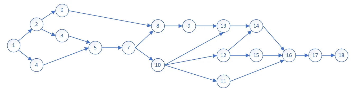
(b)

We cloud use dynamic program to solve this question, the computational process is following:

computational process of dp

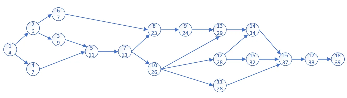
and the makespan of this project is 39 weeks

(c)

Most cost trace

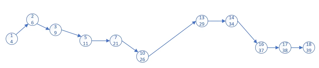
This is the most cost trace of the project, shorting each of them could save a week time.

job 7 (Walls) should be shorten most since it cost 10 weeks and all the following work must wait for its finishing.

2.4

(a)

The processor sharing is a service discipline where a number of jobs are processed simultaneously, it can be seen that the processing could be interrupt any time. For CPU, the processing already done on the preempted job is not lost, so the model of the processor sharing concept on CPU is Preemptive-Resume form.

(b)

Assume that the switch of job takes no time, there are $n$ jobs need to be processed, each job has a weight $w_j$ and process time $c_j$. Function $g(j,t)$ shows if the job $j$ has been finished on time $t$, if finished, $g(j,t)=0$; else $g(j,t)=1$. Function $f(j,t)=1$ shows that job $j$ are processed on time t, $f(j,t)=0$ shows that job $j$ are not processed on time t

We would like the cpu process the job with high weight as quickly as possible, so we get the following objective optimization problem: $$\begin{gathered} \begin{array}{}\text{(120)}& min\sum _{j=1}^n{\int }_0^{+\mathrm{\infty }}g(j,t)w_j \\ s.t.\sum _{j=1}^{n}f(j,t)\le 1 \\ g(j,t)=\{\begin{array}{lr}1& if{\int }_0^{t}f(j,\tau )d\tau \ge c_j\\ 0& otherwise\end{array} \\ {\int }_0^{+\mathrm{\infty }}f(j,\tau )d\tau =c_j\end{array} \end{gathered}$$

2.9

  jobs | 1 | 2 | 3 | 4 |
: